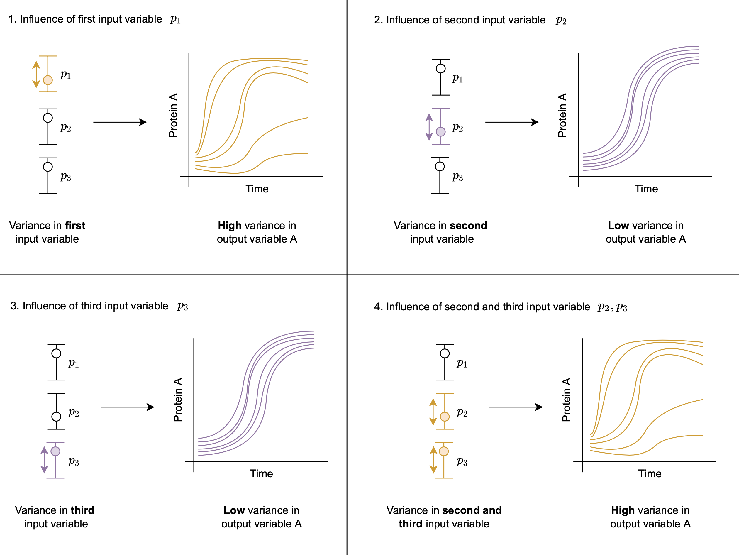
Global Sensitivity Analysis
In this tutorial, we demonstrate how to perfrom Global Sensitivity Analysis (GSA) via the Morris method in PumasQSP. This feature forms part of a rich suite of GSA tools in PumasQSP (the full list can be found here).
Julia environment
For this tutorial we will need the following packages:
| Module | Description |
|---|---|
| PumasQSP | PumasQSP is used to formulate the QSP workflow. |
| ModelingToolkit | The symbolic modeling environment |
| DifferentialEquations | The numerical differential equation solvers |
| DataSets | We will load our experimental data from datasets on JuliaHub. |
| GlobalSensitivity | We will use this for our global sensitivity analysis. |
| Plots | This is the plotting and visualization library used for this tutorial. |
Besides that we'll also need the following Julia standard libraries:
| Module | Description |
|---|---|
| Statistics | Required for the mean function |
First we prepare the environment by listing the packages we are using within the example.
# Packages used for this example
using PumasQSP
using ModelingToolkit
using DifferentialEquations
using DataSets
using GlobalSensitivity
using Statistics
using Plots
Model setup
As the example model we are using the Hires model with eight variables. Their dynamics are described by eight equations and default values are set for the variables and parameters. We use the ModelingTookit.jl package to specify the model in Julia.
# Model states and their default values
@variables begin
    t
    y1(t) = 1.0
    y2(t) = 0.0
    y3(t) = 0.0
    y4(t) = 0.0
    y5(t) = 0.0
    y6(t) = 0.0
    y7(t) = 0.0
    y8(t) = 0.0057
end

# Model parameters and their default values
@parameters begin
    k1 = 1.71
    k2 = 280.0
    k3 = 8.32
    k4 = 0.69
    k5 = 0.43
    k6 = 1.81
end

# Differential operator
D = Differential(t)

# Differential equations
eqs = [
    D(y1) ~ (-k1*y1 + k5*y2 + k3*y3 + 0.0007),
    D(y2) ~ (k1*y1 - 8.75*y2),
    D(y3) ~ (-10.03*y3 + k5*y4 + 0.035*y5),
    D(y4) ~ (k3*y2 + k1*y3 - 1.12*y4),
    D(y5) ~ (-1.745*y5 + k5*y6 + k5*y7),
    D(y6) ~ (-k2*y6*y8 + k4*y4 + k1*y5 - k5*y6 + k4*y7),
    D(y7) ~ (k2*y6*y8 - k6*y7),
    D(y8) ~ (-k2*y6*y8 + k6*y7)
]

# Model definition
@named model = ODESystem(eqs)
\[ \begin{align} \frac{\mathrm{d} \mathrm{y1}\left( t \right)}{\mathrm{d}t} =& 0.0007 + k5 \mathrm{y2}\left( t \right) + k3 \mathrm{y3}\left( t \right) - k1 \mathrm{y1}\left( t \right) \\ \frac{\mathrm{d} \mathrm{y2}\left( t \right)}{\mathrm{d}t} =& k1 \mathrm{y1}\left( t \right) - 8.75 \mathrm{y2}\left( t \right) \\ \frac{\mathrm{d} \mathrm{y3}\left( t \right)}{\mathrm{d}t} =& - 10.03 \mathrm{y3}\left( t \right) + k5 \mathrm{y4}\left( t \right) + 0.035 \mathrm{y5}\left( t \right) \\ \frac{\mathrm{d} \mathrm{y4}\left( t \right)}{\mathrm{d}t} =& - 1.12 \mathrm{y4}\left( t \right) + k3 \mathrm{y2}\left( t \right) + k1 \mathrm{y3}\left( t \right) \\ \frac{\mathrm{d} \mathrm{y5}\left( t \right)}{\mathrm{d}t} =& - 1.745 \mathrm{y5}\left( t \right) + k5 \mathrm{y6}\left( t \right) + k5 \mathrm{y7}\left( t \right) \\ \frac{\mathrm{d} \mathrm{y6}\left( t \right)}{\mathrm{d}t} =& k1 \mathrm{y5}\left( t \right) + k4 \mathrm{y4}\left( t \right) + k4 \mathrm{y7}\left( t \right) - k5 \mathrm{y6}\left( t \right) - k2 \mathrm{y6}\left( t \right) \mathrm{y8}\left( t \right) \\ \frac{\mathrm{d} \mathrm{y7}\left( t \right)}{\mathrm{d}t} =& - k6 \mathrm{y7}\left( t \right) + k2 \mathrm{y6}\left( t \right) \mathrm{y8}\left( t \right) \\ \frac{\mathrm{d} \mathrm{y8}\left( t \right)}{\mathrm{d}t} =& k6 \mathrm{y7}\left( t \right) - k2 \mathrm{y6}\left( t \right) \mathrm{y8}\left( t \right) \end{align} \]
Analysis
We create again two Trial objects and implement a reduction where the solution of the ODE system is summarised for each state. Here this is the mean for the each state and they are calculated using the Statistics package.
# Load clinical condition 1
data_1 = dataset("pumasqsptutorials/hires_trial_1")


# Creating the Trial object for trial 1
trial1 = SteadyStateTrial(data_1, model;
                        params = [k6 => 20.0],
                        alg = DynamicSS(TRBDF2()),
                        abstol = 1e-10,
                        reltol = 1e-10
)

# Clinical condition 2
data_2 = dataset("pumasqsptutorials/hires_trial_2")
trial2_params = [k3 => 4.0, k4 => 0.4, k6 => 8.0]
trial2_tspan = (0.0, 20.0)

# Creating the Trial object for trial 2
trial2 = Trial(data_2, model;
                params = trial2_params,
                tspan = trial2_tspan,
                abstol = 1e-10,
                reltol = 1e-10,
                alg = TRBDF2(),
                reduction = sol -> mean(sol, dims = 2)
)
Trial with parameters:
k3 => 4.0
k4 => 0.4
k6 => 8.0.
timespan: (0.0, 20.0)
Subsequently, we define the ranges for the parameters of the model to generate quasi-random samples using the Morris method. Lastly, we define SensitivityProblem objects, one for each trial, with the ranges of parameters to be analyzed, and perform the gsa call.
# Create SensitivityProblem
sens1 = SensitivityProblem(trial1, model,
                        [
		                k1 => (0., 5.),
 		                k2 => (200, 300)
 	                ]
)
sens2 = SensitivityProblem(trial2, model,
                        [
		                k1 => (0., 5.),
 		                k2 => (200, 300)
 	                ]
)
# Retrieve sensitivities
gsa_res1 = gsa(sens1, Morris(total_num_trajectory=1000,num_trajectory=150); batch = false, samples = 1000);
gsa_res2 = gsa(sens2, Morris(total_num_trajectory=1000,num_trajectory=150); batch = false, samples = 1000);

# Extract summary statistics
vals_first_a = gsa_res1.means
vals_first_b = gsa_res2.means
8×2 Matrix{Float64}:
-0.167146 -9.67867e-7
0.0135825 -4.64241e-7
0.00481953 -1.12902e-6
0.036909 -4.41371e-6
1.01369 -0.000284352
5.3573 -0.00146385
0.000788482 1.81553e-6
-0.000788482 -1.81553e-6Visualization
# Design Plot objects
p_first_a = bar(vals_first_a, grid = "off", ylabel = "Sensitivity ", xlabel = "States", label = "", title = "Parameter a", color = "purple")
p_total_a = bar(vals_first_b, grid = "off", ylabel = "Sensitivity ", xlabel = "States", label = "", title = "Parameter b", color = "purple")

# Show plots
plot(p_first_a, p_total_a, layout = (2,1))
Note: Instead of ranges, we can describe the respective area of the parameter space via design matrices, too. For details see GlobalSensitivity.jl.