Virtual Population: Stochastic Optimization
PumasQSP provides the methodological framework to create and use Virtual Populations (VP) in Julia. A schematical overview of a potential use case of VP generation is presented in the figure below.
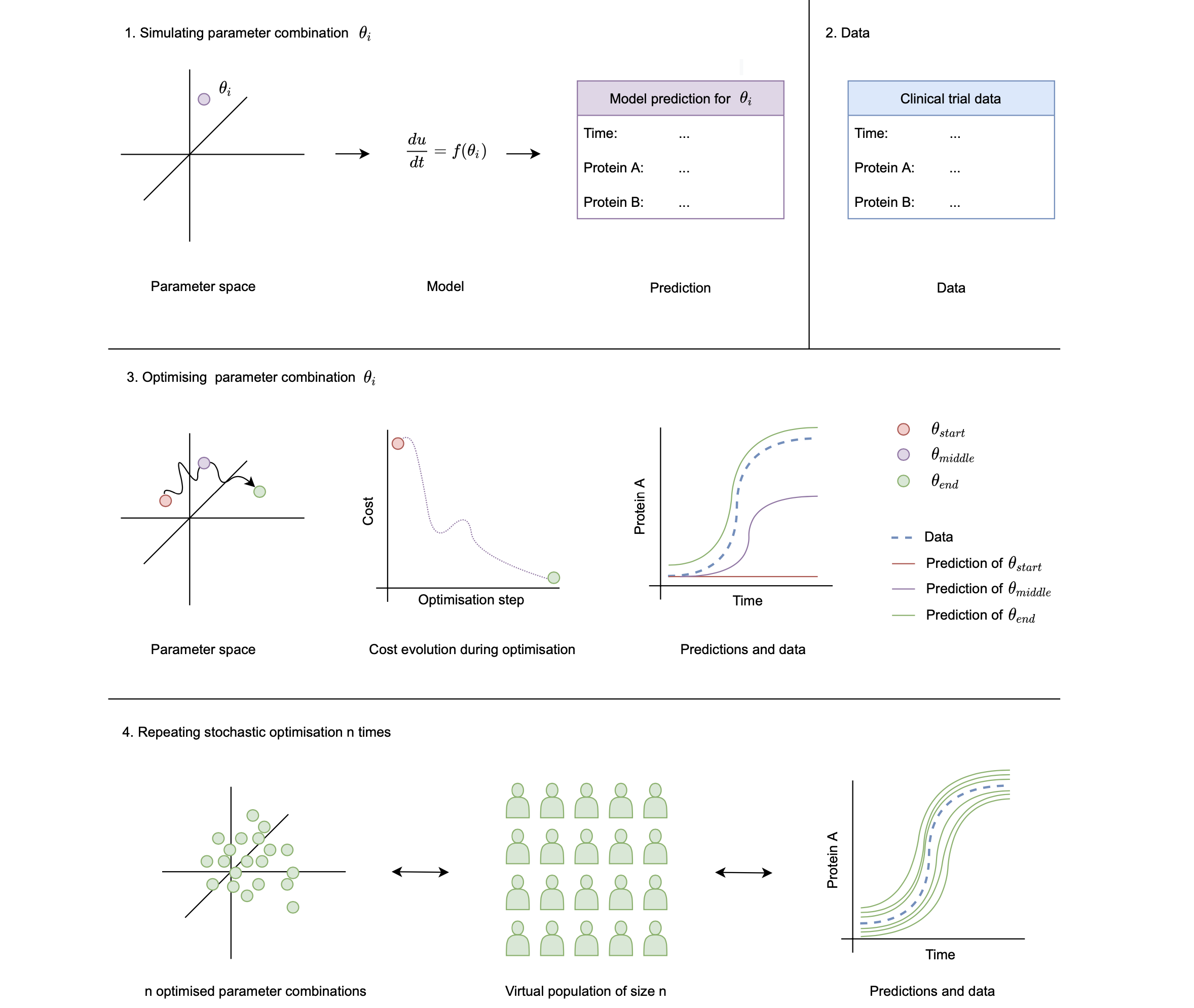
To create VPs with PumasQSP, three main ingredients are needed:
- the QSP model, i.e. the differential equations which describe the system
- the clinical trial data associated with different instantiations of the system
- some cost specifications
In this example we will showcase how to take these ingredients and generate a virutal population with parallelized stochastic optimization.
Julia environment
For this tutorial we will need the following packages:
| Module | Description |
|---|---|
| PumasQSP | PumasQSP is used to formulate the QSP workflow. |
| ModelingToolkit | The symbolic modeling environment |
| DifferentialEquations | The numerical differential equation solvers |
| DataSets | We will load our experimental data from datasets on JuliaHub. |
| DataFrames | Handling tabular data manipulation |
| Plots and StatsPlots | The plotting and visualization libraries used for this tutorial. |
First we prepare the environment by listing the packages we are using within the example.
# Packages used for this example
using PumasQSP
using ModelingToolkit
using DifferentialEquations
using DataSets
using DataFrames
using Plots
using StatsPlots
Model setup
As the example model we are using the Hires model with eight variables. Their dynamics are described by eight equations and default values are set for the variables and parameters. We use the ModelingTookit.jl package to specify the model.
# Model states and their default values
@variables begin
    t
    y1(t) = 1.0
    y2(t) = 0.0
    y3(t) = 0.0
    y4(t) = 0.0
    y5(t) = 0.0
    y6(t) = 0.0
    y7(t) = 0.0
    y8(t) = 0.0057
end

# Model parameters and their default values
@parameters begin
    k1 = 1.71
    k2 = 280.0
    k3 = 8.32
    k4 = 0.69
    k5 = 0.43
    k6 = 1.81
end

# Differential operator
D = Differential(t)

# Differential equations
eqs = [
    D(y1) ~ (-k1*y1 + k5*y2 + k3*y3 + 0.0007),
    D(y2) ~ (k1*y1 - 8.75*y2),
    D(y3) ~ (-10.03*y3 + k5*y4 + 0.035*y5),
    D(y4) ~ (k3*y2 + k1*y3 - 1.12*y4),
    D(y5) ~ (-1.745*y5 + k5*y6 + k5*y7),
    D(y6) ~ (-k2*y6*y8 + k4*y4 + k1*y5 - k5*y6 + k4*y7),
    D(y7) ~ (k2*y6*y8 - k6*y7),
    D(y8) ~ (-k2*y6*y8 + k6*y7)
]

# Model definition
@named model = ODESystem(eqs)
\[ \begin{align} \frac{\mathrm{d} \mathrm{y1}\left( t \right)}{\mathrm{d}t} =& 0.0007 + k5 \mathrm{y2}\left( t \right) + k3 \mathrm{y3}\left( t \right) - k1 \mathrm{y1}\left( t \right) \\ \frac{\mathrm{d} \mathrm{y2}\left( t \right)}{\mathrm{d}t} =& k1 \mathrm{y1}\left( t \right) - 8.75 \mathrm{y2}\left( t \right) \\ \frac{\mathrm{d} \mathrm{y3}\left( t \right)}{\mathrm{d}t} =& - 10.03 \mathrm{y3}\left( t \right) + k5 \mathrm{y4}\left( t \right) + 0.035 \mathrm{y5}\left( t \right) \\ \frac{\mathrm{d} \mathrm{y4}\left( t \right)}{\mathrm{d}t} =& - 1.12 \mathrm{y4}\left( t \right) + k3 \mathrm{y2}\left( t \right) + k1 \mathrm{y3}\left( t \right) \\ \frac{\mathrm{d} \mathrm{y5}\left( t \right)}{\mathrm{d}t} =& - 1.745 \mathrm{y5}\left( t \right) + k5 \mathrm{y6}\left( t \right) + k5 \mathrm{y7}\left( t \right) \\ \frac{\mathrm{d} \mathrm{y6}\left( t \right)}{\mathrm{d}t} =& k1 \mathrm{y5}\left( t \right) + k4 \mathrm{y4}\left( t \right) + k4 \mathrm{y7}\left( t \right) - k5 \mathrm{y6}\left( t \right) - k2 \mathrm{y6}\left( t \right) \mathrm{y8}\left( t \right) \\ \frac{\mathrm{d} \mathrm{y7}\left( t \right)}{\mathrm{d}t} =& - k6 \mathrm{y7}\left( t \right) + k2 \mathrm{y6}\left( t \right) \mathrm{y8}\left( t \right) \\ \frac{\mathrm{d} \mathrm{y8}\left( t \right)}{\mathrm{d}t} =& k6 \mathrm{y7}\left( t \right) - k2 \mathrm{y6}\left( t \right) \mathrm{y8}\left( t \right) \end{align} \]
We are considering two clinical conditions. The first trial computes a steady state which can be used as the initial condition of the second trial. First we read data and define all parameters of the first trial.
# Load data using DataSets packages
data1 = dataset("pumasqsptutorials/hires_trial_1")

trial1 = SteadyStateTrial(data1, model;
                        params = [k6 => 20.0],
                        alg = DynamicSS(QNDF()),
                        abstol = 1e-10,
                        reltol = 1e-10
)
SteadyStateTrial with parameters:
k6 => 20.0.
The second condition has altered parameters trial2_params and uses the steady state solution of trial1 as its initial value.
# Load data using DataSets package
data2 = dataset("pumasqsptutorials/hires_trial_2")

# Clinical condition 2
trial2_params = [k3 => 4.0, k4 => 0.4, k6 => 8.0]
trial2_tspan = (0.0, 20.0)

# Create the Trial object for trial 2
trial2 = Trial(data2, model;
                forward_u0 = true,
                params = trial2_params,
                tspan = trial2_tspan,
                abstol = 1e-10,
                reltol = 1e-10
)
Trial with parameters:
k3 => 4.0
k4 => 0.4
k6 => 8.0
and initial conditions obtained from another trial.
timespan: (0.0, 20.0)
Analysis
The cost function associated to the virtual population optimization problem is specified using the PumasQSP object InverseProblem. Next to the model and the trials, the user needs to specify a search space. This is to constrain the optimizer in which values to consider as potential values for the parameter combinations.
# Define a search space
example_ss = [k1 => (1.0, 3.0),
              k2 => (200.0, 400.0),
              y1 => (0.0, 3.0)
]

# Create sequence of Steady State Trials
trials = SteadyStateTrials(trial1, trial2)

# Create a InverseProblem object
prob = InverseProblem(trials, model, example_ss)
InverseProblem for model with 2 trials optimizing 3 parameters and states.
Once the QSP model and the trials are defined, the package can generate plausible patients, i.e. find parameter combinations for the provided model, which describe the trial data sufficiently well. In each optimization step, a new parameter combination is selected, the model is simulated (i.e. the ODE problem is solved) and the ODE solution is compared to the trial data to assess its fit.
# Generate potential population
vp = vpop(prob,
        StochGlobalOpt(maxiters = 750);
        population_size = 10
)
Virtual population of size 10 computed in 1 minute and 50 seconds.
┌─────────────┬─────────┬─────────┐
│ y1(t) │ k1 │ k2 │
├─────────────┼─────────┼─────────┤
│ 0.000624155 │ 1.78248 │ 355.365 │
│ 0.000614967 │ 1.70698 │ 245.446 │
│ 0.00074557 │ 1.97866 │ 283.005 │
│ 0.000708553 │ 1.62648 │ 334.92 │
│ 0.00044955 │ 1.50587 │ 256.985 │
│ 0.000590089 │ 1.56743 │ 313.256 │
│ 0.000535783 │ 1.715 │ 299.712 │
│ 0.000637378 │ 1.76005 │ 305.775 │
│ 0.000780749 │ 1.79528 │ 330.126 │
│ 0.000694205 │ 1.9734 │ 299.101 │
└─────────────┴─────────┴─────────┘
Visualization
We can conveniently analyze and visualize the results by relying on the ploting recipes for PumasQSP.
# Viusalization (1/2): Simulation results for Condition 2
plot(vp, trials[2], legend = :outerright, grid = "off")
# Viusalization (2/2): Parameters
params = DataFrame(vp)[!,"y1(t)"]
plt = violin(params, grid = :off, legend = :outerright, label = "VP", ylabel = "y1", color = "purple")
Simulating Virtual Trials
Once we have created and validated our VP, we can use it to explore the system for new clinical conditions. For this, we can use the virtual_trial function.
# Creating virtual trial
vt = virtual_trial(trials[2], model;
	                u0 = [y3 =>2.1],
	                params = [k1 => 1.9],
	                tspan = (0, 100))

# Visualize simulation results
plot(vp, vt, legend = :outerright, grid = "off")