Getting Started
Accessing PumasQSP
In order to start using the PumasQSP, you can either sign in on JuliaHub and start the PumasQSP IDE application or use the JuliaHubRegistry to download the package locally.
Using PumasQSP on JuliaHub
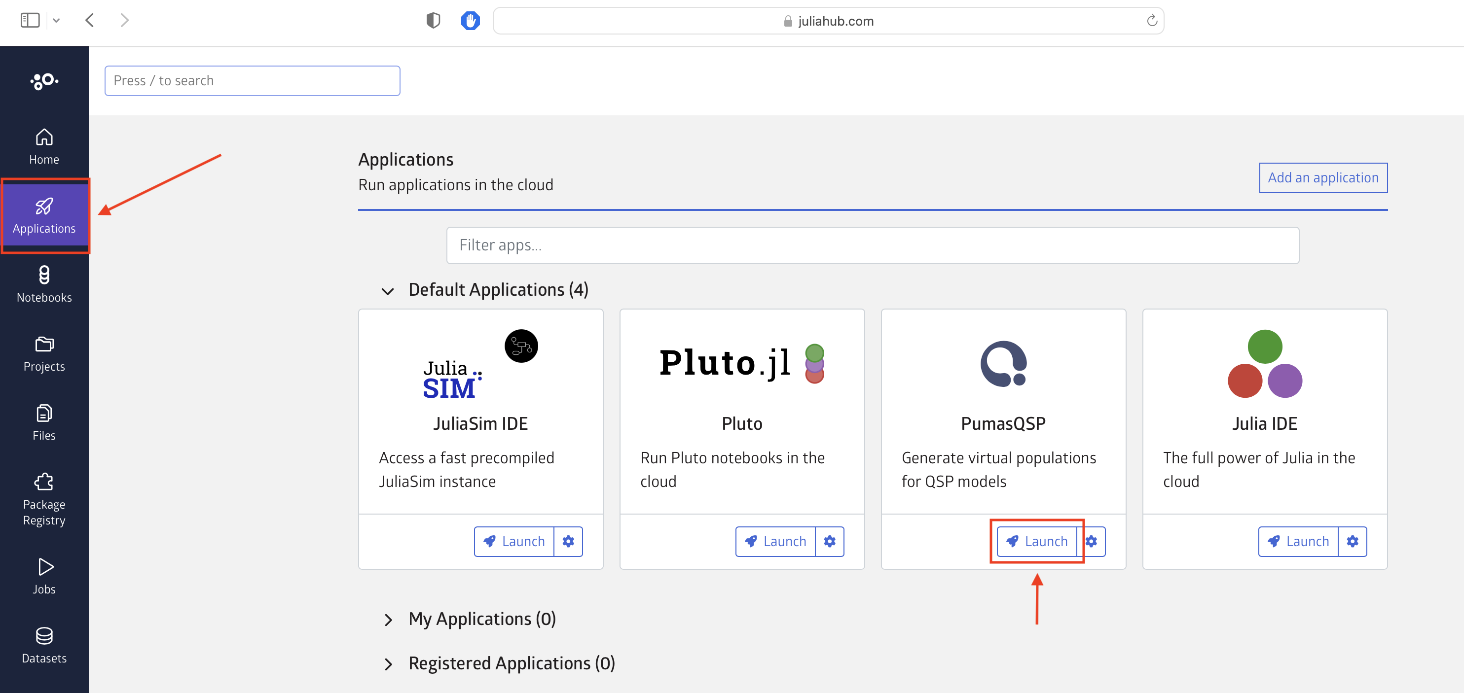
After you sign in on JuliaHub (or your JuliaHub enterprise instance), go to Applications and then start a PumasQSP app.
Using PumasQSP locally
In order to use the PumasQSP locally, you'll need to first add PkgAuthentication to your global environment.
using Pkg
original_active_project = Base.active_project()
try
  withenv("JULIA_PKG_SERVER" => nothing) do
    Pkg.activate("v$(VERSION.major).$(VERSION.minor)"; shared = true)
    Pkg.add("PkgAuthentication")
  end
finally
  Pkg.activate(original_active_project)
end
Next, configure Julia to be aware of JuliaHub's package server (or your enterprise JuliaHub instance):
using PkgAuthentication
PkgAuthentication.install("juliahub.com")
Then add all known registries on JuliaHub, including the JuliaHub registry, from the "Pkg REPL" (by pressing ] from the Julia REPL), using
Pkg.Registry.add()The command above will only work on Julia v1.8 and later. On versions prior to v1.8 use the pkg> REPL command registry add instead.
This will open up a new browser window or tab and ask you to sign in to JuliaHub or to confirm authenticating as an already logged in user.
This will also change the package server to JuliaHub for all Julia sessions that run startup.jl.
Lastly, in order to use the datasets in the tutorials, you'll have to make them accessible via JuliaHubData, so you'll have to install JuliaHubData and DataSets and then run the following.
using JuliaHubData
using DataSets
using PkgAuthentication

PkgAuthentication.authenticate()
JuliaHubData.connect_juliahub_data_project()
Fitting model parameters to data with PumasQSP
Motivation
For many of the models we work with, we do not know all the parameters. If we have experimental data available, we can calibrate the model parameters such that the simulated model behavior matches the data. In the following tutorial, we will solve the inverse problem of finding the reaction rate $k$ of the chemical reaction $A \rightarrow B$.

In the following example, we assume:
- Due to the law of mass action, the rate of change of $A$ is $\frac{dA}{dt} = -kA$.
- Due to conservation of mass, the rate of change of $B$ is $\frac{dB}{dt} = kA$.
Initial conditions are given but the parameter $k$ is unknown, and must be inferred from provided data.
Julia environment
For this getting started tutorial we will need the following packages:
| Module | Description |
|---|---|
| PumasQSP | PumasQSP is used to formulate our inverse problem and solve it |
| ModelingToolkit | The symbolic modeling environment |
| Catalyst | Provides building blocks to define chemical reaction networks compatible with MTK |
| DataSets | This is used to handle our experimental data |
| Plots | The plotting and visualization library |
First we prepare the environment by listing the packages we are using within the example.
using PumasQSP
using Catalyst
using DataSets
using Plots
Model Setup
In order to solve the inverse problem, we must first define the chemical reaction using @reaction_network from Catalyst.jl.
rn = @reaction_network begin
  @species A(t) = 10.0 B(t) = 0.0
  @parameters k = 0.5
  k, A --> B
end
model = convert(ODESystem, rn)
\[ \begin{align} \frac{\mathrm{d} A\left( t \right)}{\mathrm{d}t} =& - k A\left( t \right) \\ \frac{\mathrm{d} B\left( t \right)}{\mathrm{d}t} =& k A\left( t \right) \end{align} \]
The reaction_network syntax is very close to how chemists write reactions. First, the species present in the chemical reaction are listed, together with their initial conditions. Next, the reaction kinetic parameters are listed, together with an initial guess for their values. Finally, the reactions between these species are listed, together with the corresponding reaction rate constant. The reaction rate $k$ will be calibrated from data. The reaction network is then transformed into an ODESystem from ModelingToolkit.jl. We see that this transformation produces the equations expected from mass action.
Reading data
We read the tabular experimental data where the model names are matching column names in the table using the dataset() function of DataSets.jl. The first column is reserved for the measurement times. In this example, only the evolution in time of species $B$ is measured, but not $A$.
data = dataset("pumasqsptutorials/reaction_data")name = "pumasqsptutorials/reaction_data"
uuid = "8d99075a-7b4d-4d73-ad74-5102b16f1163"
description = "This file contains simulation data of the getting started example."
type = "Blob"
[storage]
driver = "JuliaHubDataRepo"
bucket_region = "us-east-1"
bucket = "internaljuilahubdatasets"
credentials_url = "https://internal.juliahub.com/datasets/8d99075a-7b4d-4d73-ad74-5102b16f1163/credentials"
prefix = "datasets"
vendor = "aws"
type = "Blob"
[storage.juliahub_credentials]
auth_toml_path = "/home/github_actions/actions-runner-1/home/.julia/servers/internal.juliahub.com/auth.toml"
[[storage.versions]]
blobstore_path = "u1"
date = "2023-07-25T14:14:30.249+00:00"
size = 242
version = 1
We can now create a Trial that would correspond to the experimental data above. The inverse problem is defined by the trial, the model of the system and the search space. The search space is a vector of pairs, where the first element is the model variable (parameter or initial condition) that we want to calibrate and the second represents the bounds in which we believe the value can be.
trial = Trial(data, model)
@unpack k, A = model # parameters used in search space must be unpacked from the ODESystem
search_space = [k => (0.1, 10.0)]
invprob = InverseProblem(trial , model, search_space)
InverseProblem for ##ReactionSystem#1539 with one trial optimizing 1 parameters.
Calibration
We can now calibrate the model parameters to the data using a calibration method of our choice. The simplest method that we can start with is SingleShooting.
alg = SingleShooting(maxiters = 10^4)
r = calibrate(invprob, alg)
Calibration result computed in 32 seconds. Final objective value: 1.15214e-11.
Optimization ended with Success Return Code and returned.
┌─────┐
│ k │
├─────┤
│ 0.4 │
└─────┘
To check that the result is correct, we can plot the solution of the simulated reactions to the experimental ones. To include the data in the plot, we use show_data = true. As systems can have a very large amount of states, the legend is not shown by default, so we turn that on with legend = true.
plot(trial, invprob, r, show_data = true, legend = true)