Dosing
In this tutorial, we demonstrate how to implement Bolus doses in PumasQSP Trial objects.
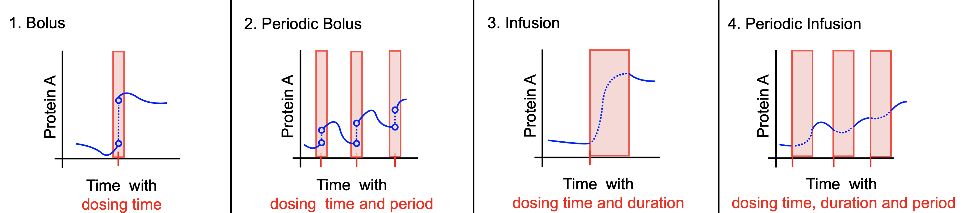
The Bolus dose forms part of a broader dosing suite including PeriodicBolus dosing, Infusion dosing and PeriodicInfusion dosing (For more details see API section). This tutorial assumes that you have read the getting started tutorial.
Julia environment
For this tutorial we will need the following packages:
| Module | Description |
|---|---|
| PumasQSP | PumasQSP is used to formulate the trial and inverse problem. |
| Catalyst | Symbolic modeling package for simulation of chemical reaction networks leveraging ModelingToolkit. |
| Plots | This is the plotting and visualization library used for this tutorial. |
First we prepare the environment by listing the packages we are using within the example.
using PumasQSP
using Catalyst
using Plots
Model setup
We use the following compartment model with two species and two parameters. We define it as a @reaction_network of Catalyst.jl and subsequently convert it to a ODESystem of ModelingToolkit.jl.
rn = @reaction_network begin
  # Define model
  @species skin(t) = 0.0 body(t) = 0.0
  @parameters kabs = 2.0 kelim = 1.0
  kabs, skin --> body
  kelim, body --> ∅
end
model  = convert(ODESystem, rn)
\[ \begin{align} \frac{\mathrm{d} \mathrm{skin}\left( t \right)}{\mathrm{d}t} =& - kabs \mathrm{skin}\left( t \right) \\ \frac{\mathrm{d} \mathrm{body}\left( t \right)}{\mathrm{d}t} =& kabs \mathrm{skin}\left( t \right) - kelim \mathrm{body}\left( t \right) \end{align} \]
The dosing feature in Trial objects
We implement two doses: one dose of 1.0 units is administered to the skin after 0.25 time units, and another dose of 0.5 units is administered after 0.75 time units. The doses are absorbed by the body by first order kinetics and are also eliminated from the body by first order kinetics. Using the unpacked species skin, we define the doses as an array of Bolus doses which allows us to increase the amount of a state, either at specific time points or at regular intervals.
# Unpack parameters and define doses
@unpack skin = model
bolus_dose_1 = Bolus(skin, 1.0, 0.25)
bolus_dose_2 = Bolus(skin, 0.5, 0.75)
bolus_doses = [bolus_dose_1, bolus_dose_2]
2-element Vector{Bolus{Symbolics.Num, Float64, Float64}}:
Bolus{Symbolics.Num, Float64, Float64}(skin(t), 1.0, 0.25)
Bolus{Symbolics.Num, Float64, Float64}(skin(t), 0.5, 0.75)This array is subseqeuntly passed to the Trial object via the doses keyword. We then create the InverseProblem, simulate the created Trial and visualize the output.
trial = Trial(model; doses = bolus_doses, saveat = 0.01,tspan = (0.0, 1.5))
prob = InverseProblem(trial, model, [])
sol = simulate(trial, prob)
plot(sol)
For more detailed information about the doses keyword see the API section.