Generating Surrogates for Parameter Estimation using an FMU Source
Motivation
Parameter estimation is a widely used technique for calibrating models to real world data. Realistic representations of industrial models can be prohibitively expensive to run the number of times required to accomplish a parameter estiamtion task. In this tutorial, we will demonstrate how to build a surrogate that will act as a high-fidelty and computationally cheap stand in for these realistic models to be used for such applications using the Coupled Clutches FMU in Co-Simulation mode.
Step by Step Walkthrough
1. Set up Surrogate Generation Environment
First we prepare the environment by importing JuliaSimSurrogates, FMI and JuliaHub
using FMI
using JuliaSimSurrogates
using JuliaHub
using JLSO
2. Loading in the FMU Simuator
Our model is in FMU form. Let's import the FMU. This can be done by giving in the path of the FMU to the fmi2Load function.
fmu = FMI.fmi2Load("Path to the CoupledClutches FMU")Model name: CoupledClutches
Type: 13. Setting up SimulatorConfig
Now that we have a working model we want to generate many samples. A collection of samples can then be used to train a surrogate model. JuliaSimSurrogates's DataGeneration submodule will help us generate the data.
Parameter Space
We will define parameter space for first two of the parameters of the FMU, while keeping the rest of the parameters fixed For defining ParameterSpace, we define the desired number of samples, bounds of the space, and labels for the parameters which is obtained from the FMU model description.
nsamples_p = 100
p_lb = [0.19, 0.39]
p_ub = [0.21, 0.41]
param_labels = FMI.FMIImport.fmi2GetParameterNames(fmu)
param_space = ParameterSpace(p_lb, p_ub, nsamples_p; labels = param_labels[1:2])
2 dimensional ParameterSpace with 100 samples
╭──────────────────┬──────────────────────────────────────────────┬──────────...
─────────╮...
│ Space Type │ Statistics │ Number...
of Samples │...
├──────────────────┼──────────────────────────────────────────────┼──────────...
─────────┤...
│ │ ╭──────────┬──────────────┬──────────────╮ │...
│ │ │ Labels │ LowerBound │ UpperBound │ │...
│ │ ├──────────┼──────────────┼──────────────┤ │...
│ │ │ T2 │ 0.19 │ 0.21 │ │...
│ ParameterSpace │ ├──────────┼──────────────┼──────────────┤ │...
│ │ │ ⋮ │ ⋮ │ ⋮ │ │...
│ │ │ ⋮ │ ⋮ │ ⋮ │ │...
│ │ ├──────────┼──────────────┼──────────────┤ │...
│ │ │ freqHz │ 0.39 │ 0.41 │ │...
│ │ ╰──────────┴──────────────┴──────────────╯ │...
╰──────────────────┴──────────────────────────────────────────────┴──────────...
─────────╯...
Simulator Configuration
In order to generate the data we now define a simulator configuration and run the simulations. This SimulatorConfig holds information about all the sampling spaces and apply them to the problem definition.
sim_config = SimulatorConfig(param_space);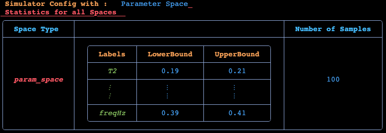
4. Deploying the Datagen Job to JuliaHub
We have defined our datagen script in the previous section, and now we will deploy the job for data generation on JuliaHub.
First we need to authenticate in JuliaHub, as this is required for submitting any batch job. This will be passed onto the function which launches the job.
auth = JuliaHub.authenticate()Now we take all the code walked through above and place it inside of @datagen
@datagen begin
  using FMI
  using JuliaSimSurrogates
  nsamples_p = 100
  p_lb = [0.19, 0.39]
  p_ub = [0.21, 0.41]
  param_labels = FMI.FMIImport.fmi2GetParameterNames(fmu)
  param_space = ParameterSpace(p_lb, p_ub, nsamples_p; labels = param_labels[1:2])
  sim_config = SimulatorConfig(param_space);
  outputs = FMI.FMIImport.fmi2GetOutputNames(fmu) .|> string

  ed = sim_config(fmu; outputs = outputs[1:3]);
end
We provide the name of the dataset where the generated data will be uploaded.
dataset_name = "coupledclutches_cs_dict""coupledclutches_cs_dict"Next, we provide the specifications of the compute required for the job: number of CPUs, GPUs, and gigabytes of memory. As a rule of thumb, we often need machines with a large number of CPUs to parallelize and scale the process of data generation.
datagen_specs = (ncpu = 4, ngpu = 0, memory = 32)(ncpu = 4, ngpu = 0, memory = 32)Next, we provide the batch image to use for the job. We will use JuliaSim image as all the packages we need can only be accessed through it.
batch_image = JuliaHub.batchimage("juliasim-batch", "JuliaSim")We then call run_datagen to launch and run the job.
datagen_job, datagen_dataset = run_datagen(@__DIR__,
   batch_image;
   auth,
   dataset_name,
   specs = datagen_specs)
Here, @__DIR__ refers to the current working directory, which gets uploaded and runs as an appbundle. This directory can be used for uploading any FMUs or other files that might be required while executing the script on the launched compute node. Any such artefacts (not part of a JuliaHub Project or Dataset) that need to be bundled must be placed in this directory.
Downloading the Dataset
Once the data generation job is finished, We can use the JuliaHub API to download our generated data.
path_datagen_dataset = JuliaHub.download_dataset(datagen_dataset, "local_path_of_the_file"; auth)We will use JLSO to deserialise it and load it as an ExperimentData.
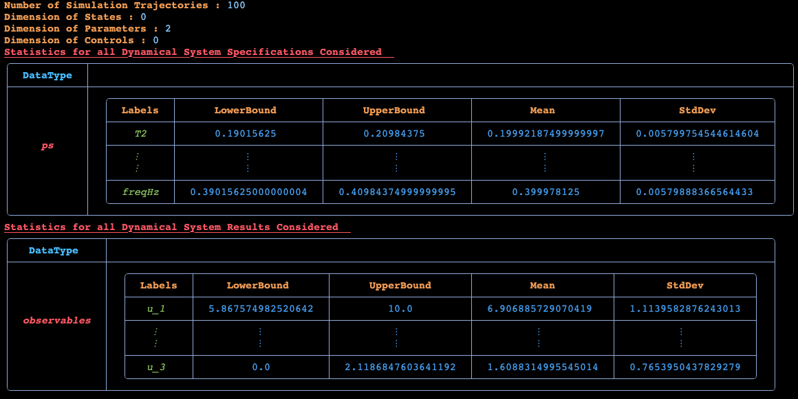
ed = ExperimentData(JLSO.load(path_datagen_dataset)[:result]) Number of Trajectories in ExperimentData: 100
Basic Statistics for Given Dynamical System's Specifications
Number of y0s in the ExperimentData: 3
Number of ps in the ExperimentData: 2
╭─────────┬──────────────────────────────────────────────────────────────────...
──╮...
│ Field │...
│...
├─────────┼──────────────────────────────────────────────────────────────────...
──┤...
│ │ ╭──────────────┬──────────────┬──────────────┬────────┬─────────...
│ │ │ Labels │ LowerBound │ UpperBound │ Mean │ StdDev...
│ │ ├──────────────┼──────────────┼──────────────┼────────┼─────────...
│ │ │ outputs[1] │ 10.0 │ 10.0 │ 10.0 │ 0.0...
│ y0s │ ├──────────────┼──────────────┼──────────────┼────────┼─────────...
│ │ │ ⋮ │ ⋮ │ ⋮ │ ⋮ │...
│ │ │ ⋮ │ ⋮ │ ⋮ │ ⋮ │...
│ │ ├──────────────┼──────────────┼──────────────┼────────┼─────────...
│ │ │ outputs[3] │ 0.0 │ 0.0 │ 0.0 │ 0.0...
│ │ ╰──────────────┴──────────────┴──────────────┴────────┴─────────...
├─────────┼──────────────────────────────────────────────────────────────────...
──┤...
│ │ ╭──────────┬──────────────┬──────────────┬────────┬──────────╮...
│ │ │ Labels │ LowerBound │ UpperBound │ Mean │ StdDev...
│ │ ├──────────┼──────────────┼──────────────┼────────┼──────────┤...
│ │ │ T2 │ 0.19 │ 0.21 │ 0.2 │ 0.006...
│ ps │ ├──────────┼──────────────┼──────────────┼────────┼──────────┤...
│ │ │ ⋮ │ ⋮ │ ⋮ │ ⋮ │ ⋮...
│ │ │ ⋮ │ ⋮ │ ⋮ │ ⋮ │ ⋮...
│ │ ├──────────┼──────────────┼──────────────┼────────┼──────────┤...
│ │ │ freqHz │ 0.39 │ 0.41 │ 0.4 │ 0.006...
│ │ ╰──────────┴──────────────┴──────────────┴────────┴──────────╯...
╰─────────┴──────────────────────────────────────────────────────────────────...
──╯...
Basic Statistics for Given Dynamical System's Continuous Fields
Number of observables in the ExperimentData: 3
╭───────────────┬────────────────────────────────────────────────────────────...
─────────╮...
│ Field │...
│...
├───────────────┼────────────────────────────────────────────────────────────...
─────────┤...
│ │ ╭──────────────┬──────────────┬──────────────┬─────────┬──...
│ │ │ Labels │ LowerBound │ UpperBound │ Mean...
│ │ ├──────────────┼──────────────┼──────────────┼─────────┼──...
│ │ │ outputs[1] │ 5.868 │ 10.0 │ 6.907...
│ observables │ ├──────────────┼──────────────┼──────────────┼─────────┼──...
│ │ │ ⋮ │ ⋮ │ ⋮ │ ⋮...
│ │ │ ⋮ │ ⋮ │ ⋮ │ ⋮...
│ │ ├──────────────┼──────────────┼──────────────┼─────────┼──...
│ │ │ outputs[3] │ 0.0 │ 2.119 │ 1.609...
│ │ ╰──────────────┴──────────────┴──────────────┴─────────┴──...
╰───────────────┴────────────────────────────────────────────────────────────...
─────────╯...
This generates an ExperimentData which can be used for fitting a DigitalEcho.
Here is a plot for the phase space of the trajectories generated.
5. Fitting a DigitalEcho
Setting up Training Script
We will use @train to write out the training script, which will be executed on the job. This is similar to data generation, where we need to write code for both importing the required packages and training a surrogate. Here, we use Surrogatize module to train a DigitalEcho.
@train begin
    using Surrogatize, Training, DataGeneration, JLSO

    ## Loading the dataset
    dict = JLSO.load(JSS_DATASET_PATH)[:result]
    ed = ExperimentData(dict)

    ## Training
    surrogate = DigitalEcho(ed;
        ground_truth_port = :observables,
        n_epochs = 24500,
        batchsize = 2048,
        lambda = 1e-7,
        tau = 1.0,
        verbose = true,
        callevery = 100)
end
Deploying the Training Job on JuliaHub
We provide the name of the dataset, which will be downloaded for us on the job and the path to it will be accessible via the environment variable JSS_DATASET_PATH. We can reference it in the training script as seen above. We also provide the name of the surrogate dataset where the trained surrogate will be uploaded.
dataset_name = "coupledclutches_cs_dict"
surrogate_name = "coupledclutches_cs_digitalecho""coupledclutches_cs_digitalecho"Next, we provide the specifications of the compute required for the job. As a rule of thumb, we need GPU machines for fitting DigitalEcho for faster training.
training_specs = (ncpu = 8, ngpu = 1, memory = 61, timelimit = 12)(ncpu = 8, ngpu = 1, memory = 61, timelimit = 12)Next, we provide the batch image to use for the job. Again, we will use JuliaSim image as all the packages we need can only be accessed through it.
batch_image = JuliaHub.batchimage("juliasim-batch", "JuliaSim")JuliaHub.BatchImage:
product: juliasim-batch
image: JuliaSim
CPU image: juliajuliasim
GPU image: juliagpujuliasimWe then call run_training to launch and run the job.
train_job, surrogate_dataset = run_training(@__DIR__,
   batch_image,
   dataset_name;
   auth,
   surrogate_name,
   specs = training_specs)
Downloading the Model
Once the training job is finished, we can download the surrogate onto our JuliaSimIDE instance to perform some validations to check whether the surrogate we trained performs well or not.
path_surrogate_dataset = JuliaHub.download_dataset(surrogate_dataset, "local_path_of_the_file"; auth)The model is serialized using JLSO, so we deserialize it:
model = JLSO.load(path)[:result]A Continous Time Surrogate wrapper with:
prob:
A `DigitalEchoProblem` with:
model:
A DigitalEcho with :
RSIZE : 256
USIZE : 3
XSIZE : 0
PSIZE : 2
ICSIZE : 0
solver: Tsit5(; stage_limiter! = trivial_limiter!, step_limiter! = trivial_limiter!, thread = static(false),)
6. Visualisation of the results
Here is a plot of the ground truth and prediction by the DigitalEcho for a trajectory in the training data