Training DigitalEcho on Battery Model from JuliaSimBatteries powered by JuliaHub
Motivation
Battery modeling is an important tool for designing and safely operating batteries in electronic devices. Simulations of physics-based battery models are computationally expensive and scale poorly with the number of connected batteries in a pack. In this tutorial, we will demonstrate how to build a surrogate that will act as a high-fidelity and computationally cheap stand-in for charging and discharging a battery pack built upon the Single Particle Model.
We will use the VSCode in our JuliaHub instance as the master node from where we run our code. This node is responsible for submitting and spawning batch jobs which actually do the computation for each of the steps in the surrogate generation pipeline.
The reason behind doing batch jobs is we can leverage the necessary compute and configurations of a node on demand for specific parts of the pipeline. These steps have specific requirements for the machines where they are executed, such as training requiring GPUs, or requiring a Windows machine. This way we optimize the cost by only paying for the platform and hardware when it's required.
Uploading and storing the result of each job is automatically handled using Datasets.
Step by Step Walkthrough
- Training DigitalEcho on Battery Model from JuliaSimBatteries powered by JuliaHub
Set up the Environment
First, we prepare the environment by importing the necessary packages on the master node.
using JuliaSimSurrogates
using JuliaSimSurrogates.JuliaHub
using JuliaSimSurrogates.JLSO
We need to authenticate in JuliaHub, as this is required for submitting any batch job. This will be passed onto the function which launches the job.
auth = JuliaHub.authenticate()Generating Data
Setting up Data Generation Script
We will use @datagen to write out the script. The script written will be submitted and executed on a separate compute node. Therefore, the script should contain both importing the required packages and also code that will generate the data.
@datagen begin
    using Random, Distributions
    using DataGeneration
    using JuliaSimBatteries
    using Controllers
    using PreProcessing

    ## Setting up the problem - 5x5 battery pack
    cell = SPM(NMC; connection = Pack(series = 5, parallel = 5), SEI_degradation = false,
        temperature = false)

    ## Setting the cell parameters
    Random.seed!(1)
    for i in 1:JuliaSimBatteries.cell_count(cell)
        setparameters(cell,
            "battery $i negative electrode active material fraction" => 0.6860102 *
                                                                        rand(Uniform(0.98,
                1.02)))
        setparameters(cell,
            "battery $i positive electrode active material fraction" => 0.6625104 *
                                                                        rand(Uniform(0.98,
                1.02)))
        setparameters(cell,
            "battery $i negative electrode thickness" => 5.62e-5rand(Uniform(0.98,
                1.02)))
        setparameters(cell,
            "battery $i positive electrode thickness" => 5.23e-5rand(Uniform(0.98,
                1.02)))
        setparameters(cell,
            "battery $i separator thickness" => 2.0e-5rand(Uniform(0.98, 1.02)))
    end

    ## Defining the controller - the parameters we got by tuning from the app
    controller = FixedICController(SIRENController(1;
            out_activation = x -> tanh.(x / 180.0),
            omega = 1 / 3),
        17.25)

    ## Defining control space
    ctrl_space = CtrlSpace(13.5, 21.0, simple_open_loop_f, 40, controller)

    ## Setting up SimulatorConfig
    simconfig = SimulatorConfig(ctrl_space)

    ## Setting up experiment
    experiment = voltage((u, p, t) -> ctrl_space.samples[1](u, t); time = 3000.0,
        bounds = false)

    ## Generating data
    ed = simconfig(cell, experiment; verbose = true,
        outputs = ["total current", "total state of charge"])
    ed_dict = PreProcessing.convert_ed_to_dict(ed)
end
Walkthrough of the Script
Defining the Battery Dynamics
For this tutorial, we will set up the script for simulating a 5x5 lithium-ion battery pack of Nickel Manganese Cobalt (NMC) chemistry using the Single Particle Model (SPM) defined in JuliaSimBatteries and use the DataGeneration module from JuliaSimSurrogates to simulate it with different inputs.
cell = SPM(NMC; connection = Pack(series = 5, parallel = 5), SEI_degradation = false,
        temperature = false)
Now, we set up the cell parameters. These parameters include:
- negative electrode active material fraction
- positive electrode active material fraction
- negative electrode thickness
- positive electrode thickness
- separator thickness
Random.seed!(1)
for i in 1:JuliaSimBatteries.cell_count(cell)
    setparameters(cell,
        "battery $i negative electrode active material fraction" => 0.6860102 *
                                                                    rand(Uniform(0.98,
            1.02)))
    setparameters(cell,
        "battery $i positive electrode active material fraction" => 0.6625104 *
                                                                    rand(Uniform(0.98,
            1.02)))
    setparameters(cell,
        "battery $i negative electrode thickness" => 5.62e-5rand(Uniform(0.98,
            1.02)))
    setparameters(cell,
        "battery $i positive electrode thickness" => 5.23e-5rand(Uniform(0.98,
            1.02)))
    setparameters(cell,
        "battery $i separator thickness" => 2.0e-5rand(Uniform(0.98, 1.02)))
end
We have defined our cell for simulation and set its parameters. For more information on defining battery dynamics, see : JuliaSimBatteries.jl. Now we need to set up our data generation configuration.
Setting up the Data Generation Configuration
We are going to demonstrate how we can simulate the battery model using inputs with partial knowledge of configuration. We define a FixedICController over a SIRENController.
The hyperparameters of the controller need tuning. See Partial Knowledge of the Configuration for more information.
controller = FixedICController(SIRENController(1;
        out_activation = x -> tanh.(x / 180.0),
        omega = 1 / 3),
    17.25)
Now we simply define a CtrlSpace with open looped controls as:
ctrl_space = CtrlSpace(13.5, 21.0, simple_open_loop_f, 40, controller)And then we define a SimulatorConfig using the above ctrl_space.
simconfig = SimulatorConfig(ctrl_space)We need to define an experiment as:
experiment = voltage((u, p, t) -> ctrl_space.samples[1](u, t); time = 3000.0,
        bounds = false)
And finally, we generate data by calling our SimulatorConfig on cell and experiment. We additionally provide keyword arguments such as outputs and verbose. outputs allow us to store certain values as observables in the ExperimentData object.
  ed = simconfig(cell, experiment; verbose = true,
      outputs = ["total current", "total state of charge"])
We additionally convert it into a julia dictionary using convert_ed_to_dict.
ed_dict = PreProcessing.convert_ed_to_dict(ed)Deploying the Datagen Job to JuliaHub
We have defined our datagen script in the previous section, and now we will deploy the job for data generation on JuliaHub. We provide the name of the dataset where the generated data will be uploaded.
dataset_name = "battery""battery"Next, we provide the specifications of the compute required for the job: number of CPUs, GPUs, and gigabytes of memory. For data generation, as a rule of thumb, we often need machines with a large number of CPUs to parallelize and scale the process.
datagen_specs = (ncpu = 4, ngpu = 0, memory = 32)(ncpu = 4, ngpu = 0, memory = 32)Next, we provide the batch image to use for the job. We will use JuliaSim image as all the packages we need can only be accessed through it.
batch_image = JuliaHub.batchimage("juliasim-batch", "JuliaSim")We then call run_datagen to launch and run the job.
datagen_job, datagen_dataset = run_datagen(@__DIR__,
   batch_image;
   auth,
   dataset_name,
   specs = datagen_specs)
Here, @__DIR__ refers to the current working directory, which gets uploaded and runs as an appbundle. This directory can be used for uploading any FMUs or other files that might be required while executing the script on the launched compute node.
Downloading the Dataset
Once the data generation job is finished, We can use the JuliaHub API to download our generated data.
path_datagen_dataset = JuliaHub.download_dataset(datagen_dataset, "local path of the file"; auth)We will use JLSO to deserialise it and load it as an ExperimentData.
ed = ExperimentData(JLSO.load(path_datagen_dataset)[:result]) Number of Trajectories in ExperimentData: 40
Basic Statistics for Given Dynamical System's Specifications
Number of u0s in the ExperimentData: 250
Number of y0s in the ExperimentData: 2
╭─────────┬──────────────────────────────────────────────────────────────────...
──────────────╮...
│ Field │...
│...
├─────────┼──────────────────────────────────────────────────────────────────...
──────────────┤...
│ │ ╭────────────────────┬──────────────┬──────────────┬────────────...
│ │...
│ │ │ Labels │ LowerBound │ UpperBound │ Mean...
│ │ │...
│ u0s │ ├────────────────────┼──────────────┼──────────────┼────────────...
│ │...
│ │ │ battery_1₊c_s[1] │ 11329.865 │ 11329.865 │ 11329.865...
│ │ │...
│ │ ├────────────────────┼──────────────┼──────────────┼────────────...
│ │...
│ ⋮ │ ⋮ │ ⋮ │ ⋮...
│...
│ ⋮ │ ⋮ │ ⋮ │ ⋮...
│...
├────────────────────┼──────────────┼──────────────┼────────────...
...
│ battery_25₊V │ 3.451 │ 3.451 │ 3.451...
│...
╰────────────────────┴──────────────┴──────────────┴────────────...
...
├─────────┼──────────────────────────────────────────────────────────────────...
──────────────┤...
│ │ ╭─────────────────────────┬──────────────┬──────────────┬───────...
│ │╮...
│ │ │ Labels │ LowerBound │ UpperBound │...
│ │ │...
│ y0s │ ├─────────────────────────┼──────────────┼──────────────┼───────...
│ │┤...
│ │ │ total current │ 9.053 │ 9.053 │...
│ │ │...
│ │ ├─────────────────────────┼──────────────┼──────────────┼───────...
│ │┤...
│ ⋮ │ ⋮ │ ⋮ │...
│...
│ ⋮ │ ⋮ │ ⋮ │...
│...
├─────────────────────────┼──────────────┼──────────────┼───────...
┤...
│ total state of charge │ 0.5 │ 0.5 │...
│...
╰─────────────────────────┴──────────────┴──────────────┴───────...
╯...
╰─────────┴──────────────────────────────────────────────────────────────────...
──────────────╯...
Basic Statistics for Given Dynamical System's Continuous Fields
Number of states in the ExperimentData: 250
Number of observables in the ExperimentData: 2
Number of controls in the ExperimentData: 1
╭───────────────┬────────────────────────────────────────────────────────────...
────────────────────╮...
│ Field │...
│...
├───────────────┼────────────────────────────────────────────────────────────...
────────────────────┤...
│ │ ╭────────────────────┬──────────────┬──────────────┬──────...
│ │╮...
│ │ │ Labels │ LowerBound │ UpperBound │...
│ │ │...
│ states │ ├────────────────────┼──────────────┼──────────────┼──────...
│ │┤...
│ │ │ battery_1₊c_s[1] │ 1670.295 │ 11329.865 │...
│ │ │...
│ │ ├────────────────────┼──────────────┼──────────────┼──────...
│ │┤...
│ ⋮ │ ⋮ │ ⋮ │...
│...
│ ⋮ │ ⋮ │ ⋮ │...
│...
├────────────────────┼──────────────┼──────────────┼──────...
┤...
│ battery_25₊V │ 3.085 │ 3.781 │...
│...
╰────────────────────┴──────────────┴──────────────┴──────...
╯...
├───────────────┼────────────────────────────────────────────────────────────...
────────────────────┤...
│ │ ╭─────────────────────────┬──────────────┬──────────────┬─...
│ │╮...
│ │ │ Labels │ LowerBound │ UpperBound...
│ │ │...
│ observables │ ├─────────────────────────┼──────────────┼──────────────┼─...
│ │┤...
│ │ │ total current │ -13.198 │ 44.769...
│ │ │...
│ │ ├─────────────────────────┼──────────────┼──────────────┼─...
│ │┤...
│ ⋮ │ ⋮ │ ⋮...
│...
│ ⋮ │ ⋮ │ ⋮...
│...
├─────────────────────────┼──────────────┼──────────────┼─...
┤...
│ total state of charge │ 0.069 │ 0.5...
│...
╰─────────────────────────┴──────────────┴──────────────┴─...
╯...
├───────────────┼────────────────────────────────────────────────────────────...
────────────────────┤...
│ │ ╭──────────┬──────────────┬──────────────┬─────────...
│ │ │ Labels │ LowerBound │ UpperBound │ Mean...
│ controls │ ├──────────┼──────────────┼──────────────┼─────────...
│ │ │ x_1 │ 15.397 │ 18.9 │ 17.255...
│ │ ╰──────────┴──────────────┴──────────────┴─────────...
╰───────────────┴────────────────────────────────────────────────────────────...
────────────────────╯...
Loading a Validation Dataset
We load in the validation data that is hosted publically on JuliaHub. This validation data is collected from real-world measurements of an electric vehicle driven around a path. We will verify our data generation process with this validation data, and later we will use it for inference. We will use the same procedure to download the dataset that we used for the training data.
validation_dataset_name = "battery_validation""battery_validation"path = JuliaHub.download_dataset(("juliasimtutorials", validation_dataset_name), "local path to the dataset")We will use JLSO to deserialize it and load it as an ExperimentData.
validation_ed = ExperimentData(JLSO.load(path_validation_dataset)[:result]) Number of Trajectories in ExperimentData: 1
Basic Statistics for Given Dynamical System's Specifications
Number of y0s in the ExperimentData: 2
╭─────────┬──────────────────────────────────────────────────────────────────...
──────────────╮...
│ Field │...
│...
├─────────┼──────────────────────────────────────────────────────────────────...
──────────────┤...
│ │ ╭─────────────────────────┬──────────────┬──────────────┬───────...
│ │╮...
│ │ │ Labels │ LowerBound │ UpperBound │...
│ │ │...
│ y0s │ ├─────────────────────────┼──────────────┼──────────────┼───────...
│ │┤...
│ │ │ total current │ 9.053 │ 9.053 │...
│ │ │...
│ │ ├─────────────────────────┼──────────────┼──────────────┼───────...
│ │┤...
│ ⋮ │ ⋮ │ ⋮ │...
│...
│ ⋮ │ ⋮ │ ⋮ │...
│...
├─────────────────────────┼──────────────┼──────────────┼───────...
┤...
│ total state of charge │ 0.5 │ 0.5 │...
│...
╰─────────────────────────┴──────────────┴──────────────┴───────...
╯...
╰─────────┴──────────────────────────────────────────────────────────────────...
──────────────╯...
Basic Statistics for Given Dynamical System's Continuous Fields
Number of observables in the ExperimentData: 2
Number of controls in the ExperimentData: 1
╭───────────────┬────────────────────────────────────────────────────────────...
────────────────────╮...
│ Field │...
│...
├───────────────┼────────────────────────────────────────────────────────────...
────────────────────┤...
│ │ ╭─────────────────────────┬──────────────┬──────────────┬─...
│ │╮...
│ │ │ Labels │ LowerBound │ UpperBound...
│ │ │...
│ observables │ ├─────────────────────────┼──────────────┼──────────────┼─...
│ │┤...
│ │ │ total current │ -1.873 │ 10.064...
│ │ │...
│ │ ├─────────────────────────┼──────────────┼──────────────┼─...
│ │┤...
│ ⋮ │ ⋮ │ ⋮...
│...
│ ⋮ │ ⋮ │ ⋮...
│...
├─────────────────────────┼──────────────┼──────────────┼─...
┤...
│ total state of charge │ 0.108 │ 0.5...
│...
╰─────────────────────────┴──────────────┴──────────────┴─...
╯...
├───────────────┼────────────────────────────────────────────────────────────...
────────────────────┤...
│ │ ╭─────────────────┬──────────────┬──────────────┬─────...
│ │ │ Labels │ LowerBound │ UpperBound │...
│ controls │ │...
│ │ ├─────────────────┼──────────────┼──────────────┼─────...
│ │ │ total voltage │ 16.37 │ 18.322 │...
│...
╰─────────────────┴──────────────┴──────────────┴─────...
╰───────────────┴────────────────────────────────────────────────────────────...
────────────────────╯...
Visualizing the Dataset
We can visualize the dataset by plotting its phase space. This gives us an idea of how well the dataset has explored the observable space.
fig, ax = plot_phase_space(ed, :observables)
fig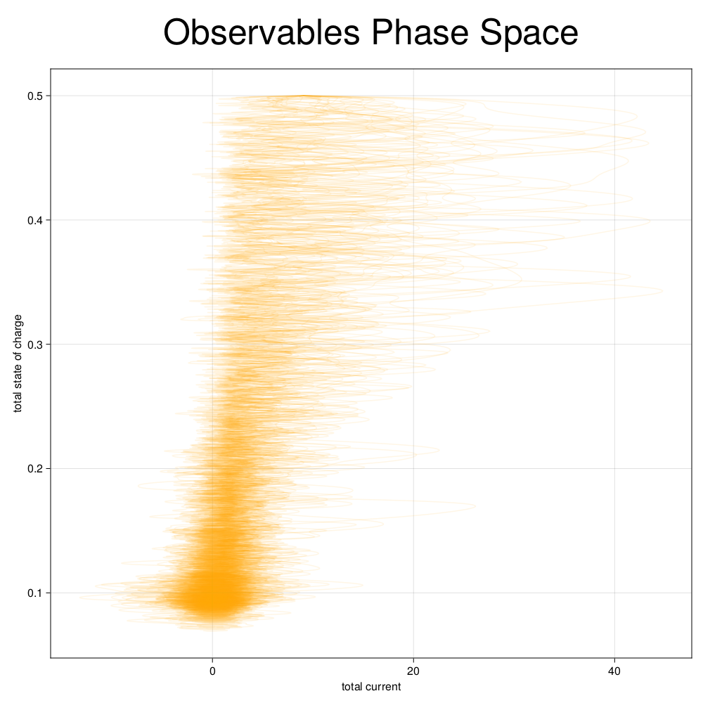 We can overlay the validation data onto the phase space to check whether the dataset was able to explore the relevant regions based on validation data.
fig, ax = plot_phase_space!(fig, ax, [validation_ed.results.observables.vals[1]])
fig
We observe that the generated dataset explores the relevant space and encloses the validation data in it as well. This indicates the data generation process could explore relevant parts of the observable space needed for real-world usage.
Next, we can plot the dataset's trajectories to confirm the expected behavior visually.
idx = 1
plot_traces(ed, idx; var_type=:observables)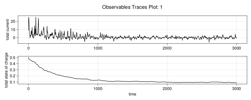
Once we ensure that we have generated data that explores the space sufficiently, we can move on to training a DigitalEcho.
Training DigitalEcho on JuliaHub
Setting up Training Script
We will use @train to write out the training script, which will be executed on the job. This is similar to data generation, where we need to write code for both importing the required packages and training a surrogate. Here, we use Surrogatize module to train a DigitalEcho.
@train begin
    using Surrogatize, DataGeneration

    ## Loading the dataset
    dict = JLSO.load(JSS_DATASET_PATH)[:result]
    ed = ExperimentData(dict)

    ## Training
    surrogate = DigitalEcho(ed;
        ground_truth_port = :observables,
        n_epochs = 24500,
        batchsize = 2048,
        lambda = 1e-7,
        tau = 1.0,
        verbose = true,
        callevery = 100)
end
Deploying the Training Job on JuliaHub
We provide the name of the dataset, which will be downloaded for us on the job and the path to it will be stored as JSS_DATASET_PATH. We can reference it in the training script as seen above. We also provide the name of the surrogate dataset where the trained surrogate will be uploaded.
dataset_name = "battery"
surrogate_name = "battery_digitalecho""battery_digitalecho"Next, we provide the specifications of the compute required for the job. As a rule of thumb, we need GPU machines for fitting DigitalEcho for faster training.
training_specs = (ncpu = 8, ngpu = 1, memory = 61, timelimit = 12)(ncpu = 8, ngpu = 1, memory = 61, timelimit = 12)Next, we provide the batch image to use for the job. Again, we will use JuliaSim image as all the packages we need can only be accessed through it.
batch_image = JuliaHub.batchimage("juliasim-batch", "JuliaSim")JuliaHub.BatchImage:
product: juliasim-batch
image: JuliaSim
CPU image: juliajuliasim
GPU image: juliagpujuliasimWe then call run_training to launch and run the job.
train_job, surrogate_dataset = run_training(@__DIR__,
   batch_image,
   dataset_name;
   auth,
   surrogate_name,
   specs = training_specs)
Downloading the Model
Once the training job is finished, we can download the surrogate onto our JuliaSimIDE instance to perform some validations to check whether the surrogate we trained performs well or not.
path_surrogate_dataset = JuliaHub.download_dataset(surrogate_dataset, "local path of the file"; auth)The model is serialized using JLSO, so we deserialize it:
model = JLSO.load(path)[:result]A Continous Time Surrogate wrapper with:
prob:
A `DigitalEchoProblem` with:
model:
A DigitalEcho with :
RSIZE : 256
USIZE : 2
XSIZE : 1
PSIZE : 0
ICSIZE : 0
solver: Tsit5(; stage_limiter! = trivial_limiter!, step_limiter! = trivial_limiter!, thread = static(false),)
Validation of the DigitalEcho
Inference on Training Data
Before inference, we need to convert the dataset into splines to get continuous controls for using it in the forward pass of the surrogate.
spline = SplineED()
ed_splines = spline(ed)
Number of Trajectories in ExperimentData: 40
Basic Statistics for Given Dynamical System's Specifications
Number of u0s in the ExperimentData: 250
Number of y0s in the ExperimentData: 2
╭─────────┬──────────────────────────────────────────────────────────────────...
──────────────╮...
│ Field │...
│...
├─────────┼──────────────────────────────────────────────────────────────────...
──────────────┤...
│ │ ╭────────────────────┬──────────────┬──────────────┬────────────...
│ │...
│ │ │ Labels │ LowerBound │ UpperBound │ Mean...
│ │ │...
│ u0s │ ├────────────────────┼──────────────┼──────────────┼────────────...
│ │...
│ │ │ battery_1₊c_s[1] │ 11329.865 │ 11329.865 │ 11329.865...
│ │ │...
│ │ ├────────────────────┼──────────────┼──────────────┼────────────...
│ │...
│ ⋮ │ ⋮ │ ⋮ │ ⋮...
│...
│ ⋮ │ ⋮ │ ⋮ │ ⋮...
│...
├────────────────────┼──────────────┼──────────────┼────────────...
...
│ battery_25₊V │ 3.451 │ 3.451 │ 3.451...
│...
╰────────────────────┴──────────────┴──────────────┴────────────...
...
├─────────┼──────────────────────────────────────────────────────────────────...
──────────────┤...
│ │ ╭─────────────────────────┬──────────────┬──────────────┬───────...
│ │╮...
│ │ │ Labels │ LowerBound │ UpperBound │...
│ │ │...
│ y0s │ ├─────────────────────────┼──────────────┼──────────────┼───────...
│ │┤...
│ │ │ total current │ 9.053 │ 9.053 │...
│ │ │...
│ │ ├─────────────────────────┼──────────────┼──────────────┼───────...
│ │┤...
│ ⋮ │ ⋮ │ ⋮ │...
│...
│ ⋮ │ ⋮ │ ⋮ │...
│...
├─────────────────────────┼──────────────┼──────────────┼───────...
┤...
│ total state of charge │ 0.5 │ 0.5 │...
│...
╰─────────────────────────┴──────────────┴──────────────┴───────...
╯...
╰─────────┴──────────────────────────────────────────────────────────────────...
──────────────╯...
Basic Statistics for Given Dynamical System's Continuous Fields
Number of states in the ExperimentData: 250
Number of observables in the ExperimentData: 2
Number of controls in the ExperimentData: 1
╭───────────────┬────────────────────────────────────────────────────────────...
────────────────────╮...
│ Field │...
│...
├───────────────┼────────────────────────────────────────────────────────────...
────────────────────┤...
│ │ ╭────────────────────┬──────────────┬──────────────┬──────...
│ │╮...
│ │ │ Labels │ LowerBound │ UpperBound │...
│ │ │...
│ states │ ├────────────────────┼──────────────┼──────────────┼──────...
│ │┤...
│ │ │ battery_1₊c_s[1] │ 1670.295 │ 11329.865 │...
│ │ │...
│ │ ├────────────────────┼──────────────┼──────────────┼──────...
│ │┤...
│ ⋮ │ ⋮ │ ⋮ │...
│...
│ ⋮ │ ⋮ │ ⋮ │...
│...
├────────────────────┼──────────────┼──────────────┼──────...
┤...
│ battery_25₊V │ 3.085 │ 3.781 │...
│...
╰────────────────────┴──────────────┴──────────────┴──────...
╯...
├───────────────┼────────────────────────────────────────────────────────────...
────────────────────┤...
│ │ ╭─────────────────────────┬──────────────┬──────────────┬─...
│ │╮...
│ │ │ Labels │ LowerBound │ UpperBound...
│ │ │...
│ observables │ ├─────────────────────────┼──────────────┼──────────────┼─...
│ │┤...
│ │ │ total current │ -13.198 │ 44.769...
│ │ │...
│ │ ├─────────────────────────┼──────────────┼──────────────┼─...
│ │┤...
│ ⋮ │ ⋮ │ ⋮...
│...
│ ⋮ │ ⋮ │ ⋮...
│...
├─────────────────────────┼──────────────┼──────────────┼─...
┤...
│ total state of charge │ 0.069 │ 0.5...
│...
╰─────────────────────────┴──────────────┴──────────────┴─...
╯...
├───────────────┼────────────────────────────────────────────────────────────...
────────────────────┤...
│ │ ╭──────────┬──────────────┬──────────────┬─────────...
│ │ │ Labels │ LowerBound │ UpperBound │ Mean...
│ controls │ ├──────────┼──────────────┼──────────────┼─────────...
│ │ │ x_1 │ 15.397 │ 18.9 │ 17.255...
│ │ ╰──────────┴──────────────┴──────────────┴─────────...
╰───────────────┴────────────────────────────────────────────────────────────...
────────────────────╯...
We will pick up a training sample from our training dataset and infer on that.
idx = 1
y0 = ed_splines.specs.y0s.vals[idx]
p = nothing
x = ed_splines.results.controls.vals[idx]
ts = ed_splines.results.tss.vals[idx]
tspan = ed_splines.specs.tspans.vals[idx]
(0.0, 3000.0)We call the forward pass of the surrogate.
pred = model(y0, (u, t) -> x(t), p, tspan; saveat = ts)2×22941 Matrix{Float64}:
9.0531 9.05338 9.05404 9.05421 … 0.134766 0.154298 0.158483
0.500031 0.500031 0.500031 0.50003 0.0887877 0.0887845 0.0887838We get the ground truth for the sample.
gt = ed.results.observables.vals[idx]2×22941 Matrix{Float64}:
9.05303 9.05422 9.05541 9.05779 … 0.134096 0.153724 0.157992
0.5 0.5 0.499999 0.499999 0.0885925 0.0885899 0.0885893Finally, we can plot to compare the prediction and the ground truth.
plot_traces(
   ts, pred, gt, ["total current", "total state of charge"]
)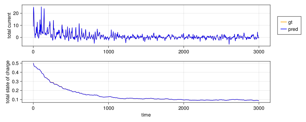
We can see the predictions and ground truth are indistinguishable. We can verify that this is "Line Over Line" performance.
Inference on Validation Data
We repeat the process above with the validation data we had loaded earlier.
spline = SplineED()
validation_ed_splines = spline(validation_ed)

idx = 1
x = validation_ed_splines.results.controls.vals[idx]
ts = validation_ed_splines.results.tss.vals[idx]
tspan = (ts[1], ts[end])
validation_pred = model(y0, (u, t) -> x(t), p, tspan; saveat = ts)
validation_gt = validation_ed.results.observables.vals[idx]
2×7623 Matrix{Float64}:
9.05303 9.05302 9.05265 9.04958 … 2.21055 2.0865 1.92479
0.5 0.5 0.5 0.499999 0.108562 0.108361 0.108174Finally, we can plot to compare the prediction and the ground truth.
plot_traces(
   ts, validation_pred, validation_gt, ["total current", "total state of charge"]
)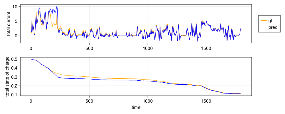
We can see that the predictions of the surrogate are great on unseen real-world data.
The above model was trained only on 40 samples for the purpose of demonstration, which is relatively small in context of training models on such complex dynamical systems. We still achieve a convincing performance and see that the model can generalize well.
Downstream Application: Real-World Comparison
Now that we have a trained DigitalEcho, we use it on real-world data:
Running Simulation on Model (left) Vs. Running DigitalEcho (right). Plots for State of Charge and Current with prediction and ground truth.
It is evident that DigitalEcho fares with high performance and unrivaled speed while maintaining accuracy in its predictions.
Generating an FMU from a DigitalEcho model
We will use @generate_fmu to write out the fmu generation script which will be executed on a separate JuliaHub job. This is important because if you want to generate a windows or linux fmu, you will need a different machine OS to do so. Writing the fmu generation script is similar to what we saw in data generation and training, where we need to write code for both importing the required packages and doing the actual work.
Setting up the FMU generation script
We provide the name of the ExperimentData dataset and the DigitalEcho dataset which will be used in the job and the path to it will be stored as JSS_DATASET_PATH and JSS_MODEL_PATH respectively. We can reference it in the FMU generation script as seen below.
@generate_fmu begin
    using Deployment, JLSO

    ed_dataset = JLSO.load(JSS_DATASET_PATH)[:result]
    ed = ExperimentData(ed_dataset)

    model = JLSO.load(JSS_MODEL_PATH)[:result]

    deploy_fmu(model, ed)
end
Deploying the FMU generation job on JuliaHub
We also provide the name of the FMU dataset where the generated FMU will be uploaded.
dataset_name = "battery"
surrogate_name = "battery_digitalecho"
fmu_name = "battery_fmu""battery_fmu"Next, we provide the specifications of the compute required for the job.
fmu_gen_specs = (ncpu = 4, ngpu = 0, memory = 32)(ncpu = 4, ngpu = 0, memory = 32)After that, we provide the batch image to use for the job. Again, we will use JuliaSim image as all the packages we need can only be accessed through it. In this case it will launch a linux machine which will generate a linux based FMU.
batch_image = JuliaHub.batchimage("juliasim-batch", "JuliaSim")JuliaHub.BatchImage:
product: juliasim-batch
image: JuliaSim
CPU image: juliajuliasim
GPU image: juliagpujuliasimWe then call run_fmu_generation to launch and run the job.
job, fmu_dataset = run_fmu_generation(@__DIR__, batchimage, surrogate_name,
    dataset_name;
    fmu_name = fmu_name, auth, specs = fmu_gen_specs, timelimit = 2)
We can choose a Windows Batch Image to generate a Windows based FMU and launch the job as well :
 win_batchimage = JuliaHub.batchimage("winworkstation-batch", "default")

job, win_fmu_dataset = run_fmu_generation(@__DIR__, win_batchimage, surrogate_name,
    dataset_name;
    fmu_name = fmu_name, auth, specs = fmu_gen_specs, timelimit = 2)
With that being done, here is the full script that takes you from data generation to deployment:
########## DATA GENERATION #########
@datagen begin
    using Random, Distributions
    using DataGeneration
    using JuliaSimBatteries
    using Controllers
    using PreProcessing

    ## Setting up the problem - 5x5 battery pack
    cell = SPM(NMC; connection = Pack(series = 5, parallel = 5), SEI_degradation = false,
        temperature = false)

    ## Setting the cell parameters
    Random.seed!(1)
    for i in 1:JuliaSimBatteries.cell_count(cell)
        setparameters(cell,
            "battery $i negative electrode active material fraction" => 0.6860102 *
                                                                        rand(Uniform(0.98,
                1.02)))
        setparameters(cell,
            "battery $i positive electrode active material fraction" => 0.6625104 *
                                                                        rand(Uniform(0.98,
                1.02)))
        setparameters(cell,
            "battery $i negative electrode thickness" => 5.62e-5rand(Uniform(0.98,
                1.02)))
        setparameters(cell,
            "battery $i positive electrode thickness" => 5.23e-5rand(Uniform(0.98,
                1.02)))
        setparameters(cell,
            "battery $i separator thickness" => 2.0e-5rand(Uniform(0.98, 1.02)))
    end

    ## Defining the controller - the parameters we got by tuning from the app
    controller = FixedICController(SIRENController(1;
            out_activation = x -> tanh.(x / 180.0),
            omega = 1 / 3),
        17.25)

    ## Defining control space
    ctrl_space = CtrlSpace(13.5, 21.0, simple_open_loop_f, 40, controller)

    ## Setting up SimulatorConfig
    simconfig = SimulatorConfig(ctrl_space)

    ## Setting up experiment
    experiment = voltage((u, p, t) -> ctrl_space.samples[1](u, t); time = 3000.0,
        bounds = false)

    ## Generating data
    ed = simconfig(cell, experiment; verbose = true,
        outputs = ["total current", "total state of charge"])
    ed_dict = PreProcessing.convert_ed_to_dict(ed)
end
dataset_name = "battery"

datagen_specs = (ncpu = 4, ngpu = 0, memory = 32)

batch_image = JuliaHub.batchimage("juliasim-batch", "JuliaSim")

datagen_job, datagen_dataset = run_datagen(@__DIR__,
   batch_image;
   auth,
   dataset_name,
   specs = datagen_specs)

########## TRAINING #########

@train begin
    using Surrogatize, DataGeneration

    ## Loading the dataset
    dict = JLSO.load(JSS_DATASET_PATH)[:result]
    ed = ExperimentData(dict)

    ## Training
    surrogate = DigitalEcho(ed;
        ground_truth_port = :observables,
        n_epochs = 24500,
        batchsize = 2048,
        lambda = 1e-7,
        tau = 1.0,
        verbose = true,
        callevery = 100)
end

surrogate_name = "battery_digitalecho"
training_specs = (ncpu = 8, ngpu = 1, memory = 61, timelimit = 12)

train_job, surrogate_dataset = run_training(@__DIR__,
   batch_image,
   dataset_name;
   auth,
   surrogate_name,
   specs = training_specs)

############ FMU GENERATION #########

@generate_fmu begin
    using Deployment, JLSO

    ed_dataset = JLSO.load(JSS_DATASET_PATH)[:result]
    ed = ExperimentData(ed_dataset)

    model = JLSO.load(JSS_MODEL_PATH)[:result]

    deploy_fmu(model, ed)
end

fmu_name = "battery_fmu"

fmu_gen_specs = (ncpu = 4, ngpu = 0, memory = 32)


job, fmu_dataset = run_fmu_generation(@__DIR__, batchimage, surrogate_name,
    dataset_name;
    fmu_name = fmu_name, auth, specs = fmu_gen_specs, timelimit = 2)