Generating Surrogates For Tuning Controllers using an ODEProblem Source
Motivation
Tuning controllers is an essential step in the design of control systems. It is however often prohibitively expensive to tune controllers for realistic models. In this tutorial, we will demonstrate how to build a surrogate that will act as a high-fidelty and computationally cheap stand in for these realistic models to be used for such applications using the Continuously Stirred Tank Reactor (CSTR) model.
Continuously Stirred Tank Reactor (CSTR) is a component model in the chemical engineering industry. It is used to model chemical reactions in a continuous flow reactor. CSTR is a nonlinear system which needs a tuned controller to acheive the desired concentrations. Hence it is a good candidate for fitting a DigitalEcho model. This model has 4 states and 2 control inputs:
States:
Cₐis the concentration of A in the reactorCᵦis the concentration of B in the reactorTᵣis the reactor temperatureTₖis the temperature of the cooling jacket
Control Inputs:
Fis the volumetric feed rateQ̇is the heat transfer rate
In this tutorial, we will fit a DigitalEcho to a CSTR ODEProblem and compare the results with the original model in both open-loop and closed-loop setting.
DigitalEchois a prorietary technique developed by JuliaHub and is available as part of JuliaSim.
Step by Step Walkthrough
1. Set up Surrogate Generation Environment
First we prepare the environment by listing the packages we are using within the example. Each package below (except for OrdinaryDiffEq) represents a module of JuliaSimSurrogates.
using OrdinaryDiffEq
using JuliaSimSurrogates
using CairoMakie
using JuliaHub
using JLSO
2. Specify the ODE Problem
We first specify the CSTR model as a function of the form f(u, x, p, t) where
uis the states of the system,xis the control inputs,pis the parameters of the system andtis the time.
The function returns the derivative of the states.
function cstr(u, x, p, t)
    Cₐ, Cᵦ, Tᵣ, Tₖ = u
    F, Q̇ = x
    [
        (5.1 - Cₐ) * F - 1.287e12Cₐ * exp(-9758.3 / (273.15 + Tᵣ)) -
        9.043e9exp(-8560.0 / (273.15 + Tᵣ)) * abs2(Cₐ),
        1.287e12Cₐ * exp(-9758.3 / (273.15 + Tᵣ)) - Cᵦ * F -
        1.287e12Cᵦ * exp(-9758.3 / (273.15 + Tᵣ)),
        30.828516377649326(Tₖ - Tᵣ) + (130.0 - Tᵣ) * F -
        0.35562611177613196(5.4054e12Cₐ * exp(-9758.3 / (273.15 + Tᵣ)) -
                            1.4157e13Cᵦ * exp(-9758.3 / (273.15 + Tᵣ)) -
                            3.7844955e11exp(-8560.0 / (273.15 + Tᵣ)) * abs2(Cₐ)),
        0.1(866.88(Tᵣ - Tₖ) + Q̇),
    ]
end
cstr (generic function with 1 method)Next, we specify the initial conditions u0 and the time span tspan for the simulation. This system does not have any parameters, so we set p to nothing.
We import OrdinaryDiffEq.jl which will allow us to define the ODEProblem.
u0 = [0.8, 0.5, 134.14, 130.0]
tspan = (0.0, 0.25)
p = nothing
prob = ODEProblem{false}(cstr, u0, tspan, p)
ODEProblem with uType Vector{Float64} and tType Float64. In-place: false
timespan: (0.0, 0.25)
u0: 4-element Vector{Float64}:
0.8
0.5
134.14
130.03. Setting up SimulatorConfig
We use the SimulatorConfig to define the control space for the CSTR model.
We specify the lower and upper bounds for the control inputs F and Q̇.
controls_lb = [5, -8500]
controls_ub = [100, 0.0]
2-element Vector{Float64}:
100.0
0.0We define the number of samples to be generated in the control space along with their labels. We also specify the number of states in the system that the closed-loop controller should expect.
nsamples = 1000
labels = ["F", "Q̇"]
n_states = length(u0)4We use RandomNeuralController which is an in-house data generation strategy for component surrogates. on AbstractController.
alg = RandomNeuralController(1,
    out_activation = x -> sin(x * 4),
    hidden_activation = x -> sin(x));
We use the simple_closed_loop_f function to specify that we want to use closed feedback controllers as part of the data generation strategy
ctrl_space = CtrlSpace(controls_lb, controls_ub, simple_open_loop_f, nsamples, alg;
    labels);
We use the SimulatorConfig to define data generation space for the CSTR model.
sim_config = SimulatorConfig(ctrl_space);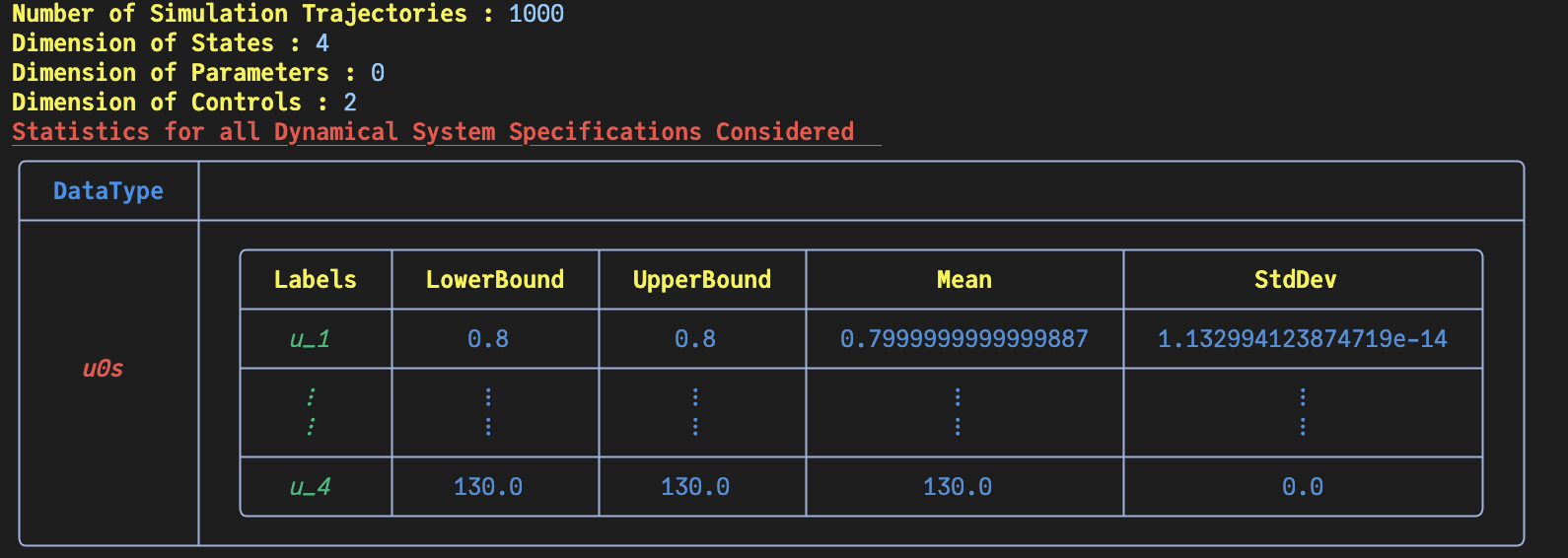
4. Deploying the Datagen Job to JuliaHub
We have defined our datagen script in the previous section, and now we will deploy the job for data generation on JuliaHub. This is done using the @datagen macro.
First we need to authenticate in JuliaHub, as this is required for submitting any batch job. This will be passed onto the function which launches the job.
auth = JuliaHub.authenticate()Now we take all the code walked through above and place it inside of @datagen
@datagen begin
    using OrdinaryDiffEq
    using JuliaSimSurrogates
    function cstr(u, x, p, t)
        Cₐ, Cᵦ, Tᵣ, Tₖ = u
        F, Q̇ = x
        [
            (5.1 - Cₐ) * F - 1.287e12Cₐ * exp(-9758.3 / (273.15 + Tᵣ)) -
            9.043e9exp(-8560.0 / (273.15 + Tᵣ)) * abs2(Cₐ),
            1.287e12Cₐ * exp(-9758.3 / (273.15 + Tᵣ)) - Cᵦ * F -
            1.287e12Cᵦ * exp(-9758.3 / (273.15 + Tᵣ)),
            30.828516377649326(Tₖ - Tᵣ) + (130.0 - Tᵣ) * F -
            0.35562611177613196(5.4054e12Cₐ * exp(-9758.3 / (273.15 + Tᵣ)) -
                                1.4157e13Cᵦ * exp(-9758.3 / (273.15 + Tᵣ)) -
                                3.7844955e11exp(-8560.0 / (273.15 + Tᵣ)) * abs2(Cₐ)),
            0.1(866.88(Tᵣ - Tₖ) + Q̇),
        ]
    end
    u0 = [0.8, 0.5, 134.14, 130.0]
    tspan = (0.0, 0.25)
    p = nothing
    prob = ODEProblem{false}(cstr, u0, tspan, p)
    controls_lb = [5, -8500]
    controls_ub = [100, 0.0]
    nsamples = 1000
    labels = ["F", "Q̇"]
    n_states = length(u0)
    alg = RandomNeuralController(1,
        out_activation = x -> sin(x * 4),
        hidden_activation = x -> sin(x));
    ctrl_space = CtrlSpace(controls_lb, controls_ub, simple_open_loop_f, nsamples, alg;
        labels);
    sim_config = SimulatorConfig(ctrl_space);
    ed = sim_config(prob; reltol = 1e-8, abstol = 1e-8);
end
We provide the name of the dataset where the generated data will be uploaded.
dataset_name = "cstr""cstr"Next, we provide the specifications of the compute required for the job: number of CPUs, GPUs, and gigabytes of memory. For data generation, as a rule of thumb, we often need machines with a large number of CPUs to parallelize and scale the process.
datagen_specs = (ncpu = 4, ngpu = 0, memory = 32)(ncpu = 4, ngpu = 0, memory = 32)Next, we provide the batch image to use for the job. We will use JuliaSim image as all the packages we need can only be accessed through it.
batch_image = JuliaHub.batchimage("juliasim-batch", "JuliaSim")We then call run_datagen to launch and run the job.
datagen_job, datagen_dataset = run_datagen(@__DIR__,
   batch_image;
   auth,
   dataset_name,
   specs = datagen_specs)
Here, @__DIR__ refers to the current working directory, which gets uploaded and runs as an appbundle. This directory can be used for uploading any FMUs or other files that might be required while executing the script on the launched compute node. Any such artefacts (not part of a JuliaHub Project or Dataset) that need to be bundled must be placed in this directory.
Downloading the Dataset
Once the data generation job is finished, We can use the JuliaHub API to download our generated data.
path_datagen_dataset = JuliaHub.download_dataset(datagen_dataset, "local_path_of_the_file"; auth)We will use JLSO to deserialise it and load it as an ExperimentData.
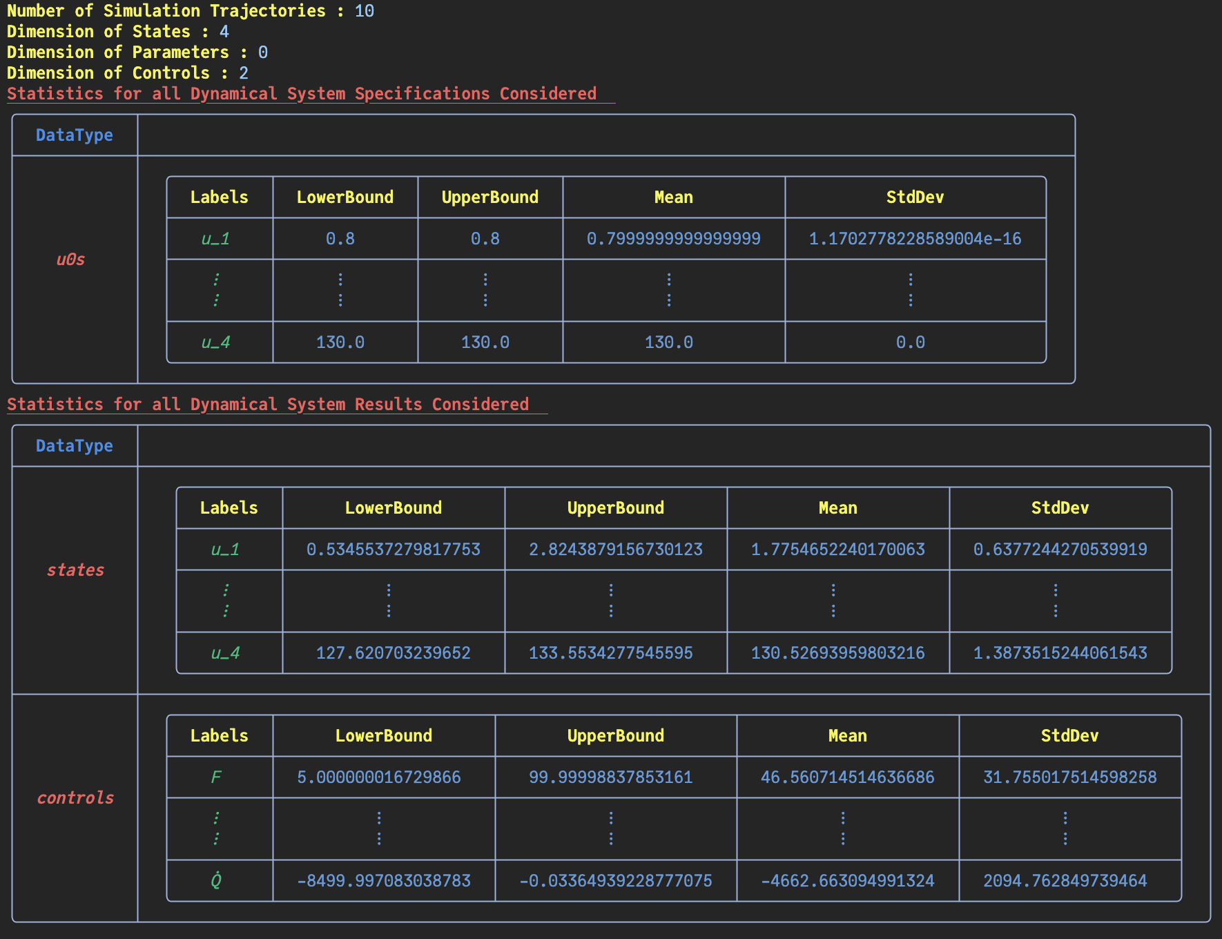
ed = ExperimentData(JLSO.load(path_datagen_dataset)[:result]) Number of Trajectories in ExperimentData: 10
Basic Statistics for Given Dynamical System's Specifications
Number of u0s in the ExperimentData: 4
╭─────────┬──────────────────────────────────────────────────────────────────...
─╮...
│ Field │...
│...
├─────────┼──────────────────────────────────────────────────────────────────...
─┤...
│ │ ╭────────────┬──────────────┬──────────────┬─────────┬──────────...
│ │ │ Labels │ LowerBound │ UpperBound │ Mean │ StdDev...
│ │ ├────────────┼──────────────┼──────────────┼─────────┼──────────...
│ │ │ states_1 │ 0.8 │ 0.8 │ 0.8 │ 0.0...
│ u0s │ ├────────────┼──────────────┼──────────────┼─────────┼──────────...
│ │ │ ⋮ │ ⋮ │ ⋮ │ ⋮ │ ⋮...
│ │ │ ⋮ │ ⋮ │ ⋮ │ ⋮ │ ⋮...
│ │ ├────────────┼──────────────┼──────────────┼─────────┼──────────...
│ │ │ states_4 │ 130.0 │ 130.0 │ 130.0 │ 0.0...
│ │ ╰────────────┴──────────────┴──────────────┴─────────┴──────────...
╰─────────┴──────────────────────────────────────────────────────────────────...
─╯...
Basic Statistics for Given Dynamical System's Continuous Fields
Number of states in the ExperimentData: 4
Number of controls in the ExperimentData: 2
╭────────────┬───────────────────────────────────────────────────────────────...
────────╮...
│ Field │...
│...
├────────────┼───────────────────────────────────────────────────────────────...
────────┤...
│ │ ╭────────────┬──────────────┬──────────────┬───────────┬────...
│ │ │ Labels │ LowerBound │ UpperBound │ Mean...
│ │ ├────────────┼──────────────┼──────────────┼───────────┼────...
│ │ │ states_1 │ 0.782 │ 2.694 │ 2.02...
│ states │ ├────────────┼──────────────┼──────────────┼───────────┼────...
│ │ │ ⋮ │ ⋮ │ ⋮ │ ⋮...
│ │ │ ⋮ │ ⋮ │ ⋮ │ ⋮...
│ │ ├────────────┼──────────────┼──────────────┼───────────┼────...
│ │ │ states_4 │ 125.364 │ 139.993 │ 131.565...
│ │ ╰────────────┴──────────────┴──────────────┴───────────┴────...
├────────────┼───────────────────────────────────────────────────────────────...
────────┤...
│ │ ╭──────────┬──────────────┬──────────────┬─────────────┬─────...
│ │ │ Labels │ LowerBound │ UpperBound │ Mean │...
│ │ ├──────────┼──────────────┼──────────────┼─────────────┼─────...
│ │ │ F │ 8.333 │ 99.468 │ 55.896 │...
│ controls │ ├──────────┼──────────────┼──────────────┼─────────────┼─────...
│ │ │ ⋮ │ ⋮ │ ⋮ │ ⋮ │...
│ │ │ ⋮ │ ⋮ │ ⋮ │ ⋮ │...
│ │ ├──────────┼──────────────┼──────────────┼─────────────┼─────...
│ │ │ Q̇ │ -8497.874 │ -227.416 │ -4158.499 │...
│ │ ╰──────────┴──────────────┴──────────────┴─────────────┴─────...
╰────────────┴───────────────────────────────────────────────────────────────...
────────╯...
This return an ExperimentData object.
5. Visualizing the generated data
We can visualize the generated data in phase space of the states of the system. We would want to choose RandomNeuralController hyperparameters which would generate data that covers the entire phase space of interest of the system.
fig, ax = plot_phase_space(ed, :states)
fig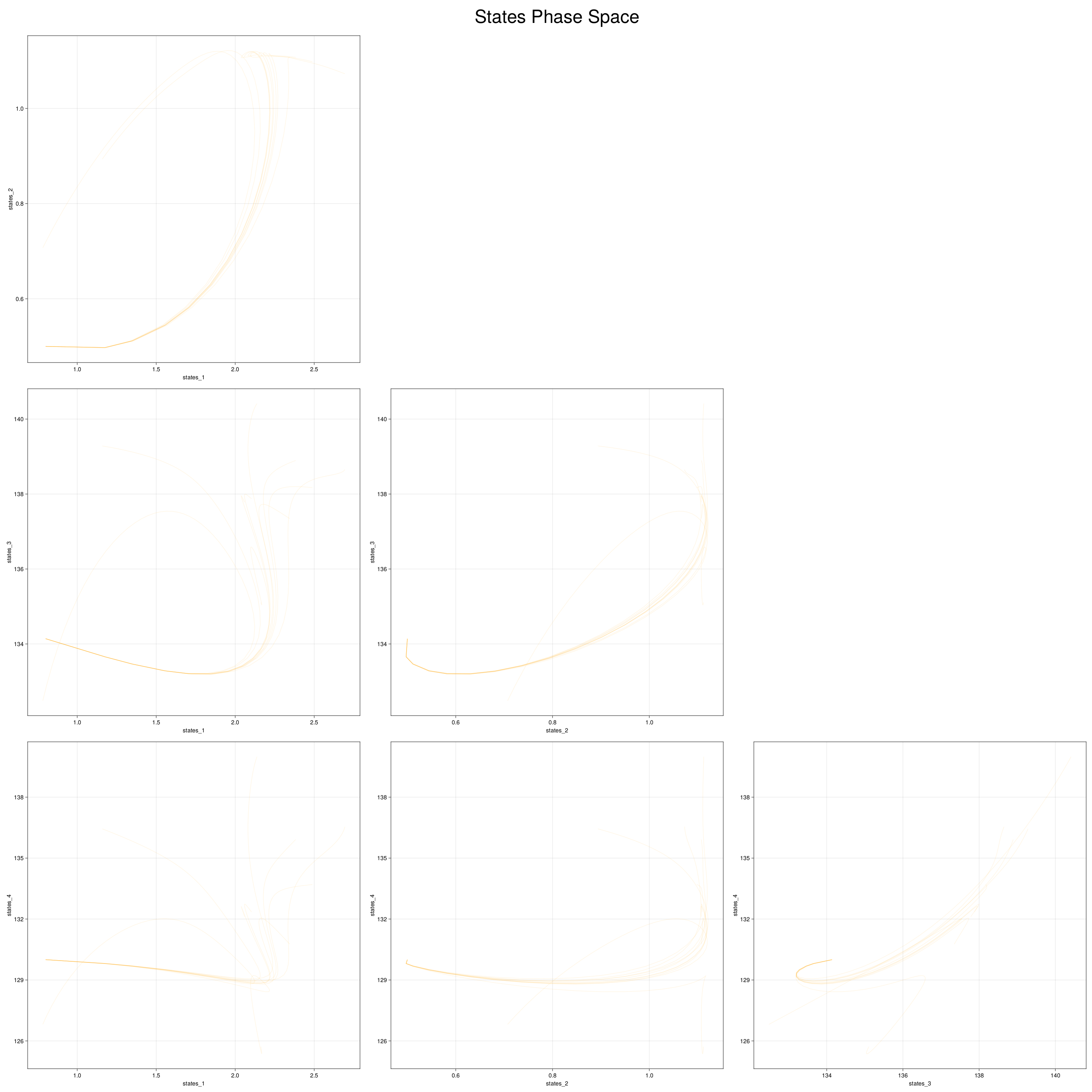
We can also visualize the generated data in phase space of the control inputs of the system. We would want to make sure that the generated data covers the entire control space of interest.
fig, ax = plot_phase_space(ed, :controls)
fig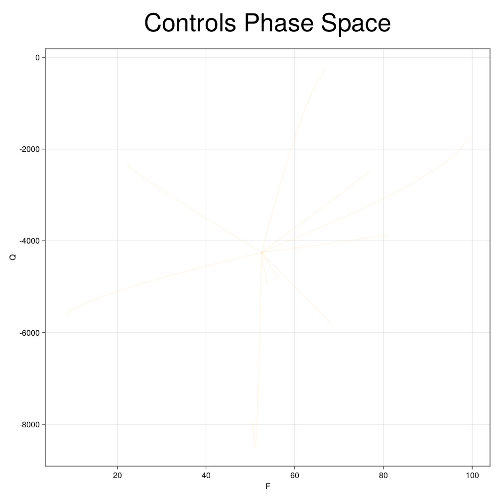
Here is a visualization of the generated data in phase space of the states of the system: 
6. Fitting a DigitalEcho
Setting up Training Script
We will use @train to write out the training script, which will be executed on the job. This is similar to data generation, where we need to write code for both importing the required packages and training a surrogate. Here, we use Surrogatize module to train a DigitalEcho.
@train begin
    using Surrogatize, Training, DataGeneration, JLSO

    ## Loading the dataset
    dict = JLSO.load(JSS_DATASET_PATH)[:result]
    ed = ExperimentData(dict)

    ## Training
    surrogate = DigitalEcho(ed;
        ground_truth_port = :states,
        n_epochs = 24500,
        batchsize = 2048,
        lambda = 1e-7,
        tau = 1.0,
        verbose = true,
        callevery = 100)
end
Deploying the Training Job on JuliaHub
We provide the name of the dataset, which will be downloaded for us on the job and the path to it will be accessible via the environment variable JSS_DATASET_PATH. We can reference it in the training script as seen above. We also provide the name of the surrogate dataset where the trained surrogate will be uploaded.
dataset_name = "cstr"
surrogate_name = "cstr_digitalecho""cstr_digitalecho"Next, we provide the specifications of the compute required for the job. As a rule of thumb, we need GPU machines for fitting DigitalEcho for faster training.
training_specs = (ncpu = 8, ngpu = 1, memory = 61, timelimit = 12)(ncpu = 8, ngpu = 1, memory = 61, timelimit = 12)Next, we provide the batch image to use for the job. Again, we will use JuliaSim image as all the packages we need can only be accessed through it.
batch_image = JuliaHub.batchimage("juliasim-batch", "JuliaSim")JuliaHub.BatchImage:
product: juliasim-batch
image: JuliaSim
CPU image: juliajuliasim
GPU image: juliagpujuliasimWe then call run_training to launch and run the job.
train_job, surrogate_dataset = run_training(@__DIR__,
   batch_image,
   dataset_name;
   auth,
   surrogate_name,
   specs = training_specs)
Downloading the Model
Once the training job is finished, we can download the surrogate onto our JuliaSimIDE instance to perform some validations to check whether the surrogate we trained performs well or not.
path_surrogate_dataset = JuliaHub.download_dataset(surrogate_dataset, "local_path_of_the_file"; auth)The model is serialized using JLSO, so we deserialize it:
model = JLSO.load(path)[:result]A Continous Time Surrogate wrapper with:
prob:
A `DigitalEchoProblem` with:
model:
A DigitalEcho with :
RSIZE : 256
USIZE : 4
XSIZE : 2
PSIZE : 0
ICSIZE : 0
solver: Tsit5(; stage_limiter! = trivial_limiter!, step_limiter! = trivial_limiter!, thread = static(false),)
7. Visualization
Here is the visualization of the overfit on 10 trajectories 
8. Results with n_epochs=14000 and nsamples=1000

Here are some validation results that demonstrate the effectiveness of the surrogate to generalize to data it hasn't seen before when the number of trajectories to be sampled are increased to 1000. Note that yellow here represents the original model and blue represents the surrogate model.
Closed Loop Controller
We validated our surrogate model in closed-loop control setting on held-out validations data generated using the random neural controllers: 
Open Loop Controller
We validated our surrogate model in open-loop control setting on independently generated MPC controller data. This data was generated separate from the data used to train the model and is different qualitatively from the training data. But the model continues to do well in this setting: