Generating Surrogates for Model Discovery using a Dataset source

Motivation

Model Discovery is a widely used technique to identify data-driven models from data In this tutorial, we will demonstrate how to build a surrogate that will act as a high-fidelty and computationally cheap stand in for these realistic models to be used for such applications using a control driven Lotka Volterra system.

Introduction

Lotka Volterra equations are usually used to govern the dynamics of biological systems of how predator-prey species react in an ecosystem. The system has a set of parameters α, β, γ, δ, and the dataset drive the system using paramaterized control functions. $ \frac{dx}{dt} = \alpha x - \beta xy + x1 $ $ \frac{dy}{dt} = \delta y - \gamma xy - x2 $

Step by Step Walkthrough

1. Set up Surrogate Generation Environment

We start by importing the required packages.

using JuliaSimSurrogates
using DataSets
using BSON
using JuliaHub
using JLSO

2. Loading in your dataset.

We load the dataset. The dataset should be in the form compatible with the supported format.

ExperimentData(dict::AbstractDict)

* "states_labels": Vector{String},
* "states": Vector{Matrix{Float64}} with every element matrix being size (state_num, time_num)
* "observables_labels": Vector{String},
* "observables": Vector{Matrix{Float64}} with every element matrix being size (observable_num, time_num)
* "params_labels": Vector{String} every element corresponds to the name of a parameter
* "params": Vector{Vector{Float64}} with every element being a vector of real values
* "controls_labels": Vector{String} every element corresponds to the name of a control
* "controls": Vector{Matrix} where every element matrix of shape (state_num, time_num)
* "ts": Vector{Vector} where every element is a vector of real values corresponding to the time steps the simulation was evaluated at

BSON.jl is a serialization package. Passing the path to the serialized file, will load a julia dictionary that has our dataset. We load a dataset that is hosted publically from JuliaHub. We load the dataset using JuliaHub.jl API.

dataset_name = "lotka_volterra_surrogates"
train_dataset = JuliaHub.dataset(("juliasimtutorials", dataset_name))

Dataset: lotka_volterra_surrogates (Blob)
 owner: juliasimtutorials
 description: A dataset of the collected data on simulating a Lotka-Volterra model with controls and parameters in JSS format to surrogatize using DigitalEcho. 
 versions: 2
 size: 160313 bytes

We now download this dataset reference to a local directory.

path = JuliaHub.download_dataset(train_dataset, "../assets/lv_dataset.bson")

"/home/github_actions/actions-runner-1/_work/JuliaSimSurrogates.jl/JuliaSimSurrogates.jl/docs/build/assets/lv_dataset.bson"

And now load the dataset using BSON.jl

data = BSON.load(path)

Dict{String, Union{Nothing, Vector}} with 9 entries:
  "params_labels"      => Any["p_1", "p_2", "p_3", "p_4"]
  "controls"           => Any[[-1.05879e-22 0.00143396 … -0.00528374 -0.0012435…
  "states_labels"      => Any["u_1", "u_2"]
  "controls_labels"    => Any["x_1", "x_2"]
  "observables"        => nothing
  "params"             => Any[[1.875, 1.84375, 2.125, 1.96875], [1.875, 1.84375…
  "states"             => Any[[1.0 1.00329 … 1.00583 0.999657; 1.0 0.988241 … 1…
  "ts"                 => Any[[0.0, 0.0765528, 0.227967, 0.414242, 0.607024, 0.…
  "observables_labels" => nothing

3. Generate ExperimentData from this dataset.

ed = ExperimentData(data);

We can see the summary of the ExperimentData here: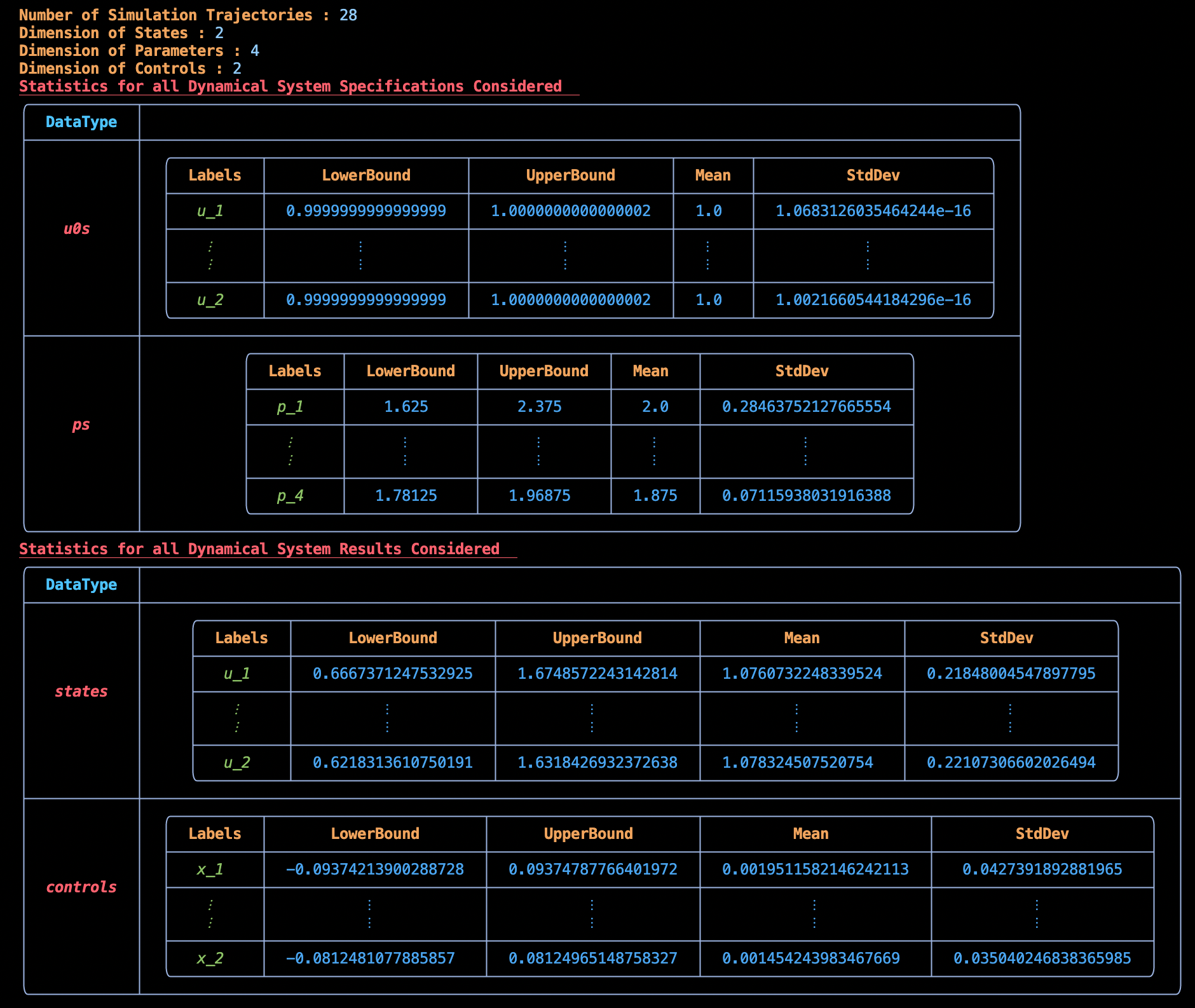

4. Fitting a DigitalEcho

For fitting the above system on our ExperimentData object we use DigitalEcho from Surrogatize. Note that we are training on states here. If we were to train on observables we can set it by passing ground_truth_port = :observables in kwargs.

Setting up Training Script

We will use @train to write out the training script, which will be executed on the job. This is similar to data generation, where we need to write code for both importing the required packages and training a surrogate. Here, we use Surrogatize module to train a DigitalEcho.

@train begin
    using Surrogatize, Training, DataGeneration, JLSO

    ## Loading the dataset
    dict = JLSO.load(JSS_DATASET_PATH)[:result]
    ed = ExperimentData(dict)

    ## Training
    surrogate = DigitalEcho(ed;
        ground_truth_port = :states,
        n_epochs = 24500,
        batchsize = 2048,
        lambda = 1e-7,
        tau = 1.0,
        verbose = true,
        callevery = 100)
end

Deploying the Training Job on JuliaHub

We provide the name of the dataset, which will be downloaded for us on the job and the path to it will be accessible via the environment variable JSS_DATASET_PATH. We can reference it in the training script as seen above.

First we need to authenticate in JuliaHub, as this is required for submitting any batch job. This will be passed onto the function which launches the job.

auth = JuliaHub.authenticate()

We also provide the name of the surrogate dataset where the trained surrogate will be uploaded.

dataset_name = "lotka_volterra_surrogates"
surrogate_name = "lotka_volterra_digitalecho"

"lotka_volterra_digitalecho"

Next, we provide the specifications of the compute required for the job. As a rule of thumb, we need GPU machines for fitting DigitalEcho for faster training.

training_specs = (ncpu = 8, ngpu = 1, memory = 61, timelimit = 12)

(ncpu = 8, ngpu = 1, memory = 61, timelimit = 12)

Next, we provide the batch image to use for the job. Again, we will use the JuliaSim image as all the packages we need can only be accessed through it.

batch_image = JuliaHub.batchimage("juliasim-batch", "JuliaSim")

JuliaHub.BatchImage: 
 product: juliasim-batch
 image: JuliaSim
 CPU image: juliajuliasim
 GPU image: juliagpujuliasim

We then call run_training to launch and run the job.

train_job, surrogate_dataset = run_training(@__DIR__,
   batch_image,
   dataset_name;
   auth,
   surrogate_name,
   specs = training_specs)

Downloading the Model

Once the training job is finished, we can download the surrogate onto our JuliaSimIDE instance to perform some validations to check whether the surrogate we trained performs well or not.

path_surrogate_dataset = JuliaHub.download_dataset(surrogate_dataset, "local_path_of_the_file"; auth)

The model is serialized using JLSO, so we deserialize it:

model = JLSO.load(path)[:result]

A Continous Time Surrogate wrapper with:
prob:
  A `DigitalEchoProblem` with:
  model:
    A DigitalEcho with : 
      RSIZE : 256
      USIZE : 2
      XSIZE : 0
      PSIZE : 4
      ICSIZE : 0
solver: Tsit5(; stage_limiter! = trivial_limiter!, step_limiter! = trivial_limiter!, thread = static(false),)

Here are some plots for the trajectories generated against ground truth.