Generating a DigitalEcho for the Brusselator Model Powered by JuliaHub
Motivation
The Brusselator is a well-known model for describing oscillations in chemical reactions. This model involves a system of highly stiff Partial Differential Equations (PDEs) which is very difficult to simulate and scales poorly with increasing discretization.
This tutorial will demonstrate how to build a surrogate that will act as a high-fidelty and computationally cheap stand-in for the 2D Brusselator model.
We will use the JuliaSim IDE as the master node to spawn jobs on JuliaHub for generating data and then use it for our DigitalEcho pipeline.
Step by Step Walkthrough
This tutorial will demonstrate an end-to-end example of training DigitalEcho for the Brusselator model. This tutorial will be divided into the following subsections:
- Generating a DigitalEcho for the Brusselator Model Powered by JuliaHub
Setting up the Environment
In order to set up the environment, we need to import JuliaSimSurrogates in the environment. We include JLSO for deserialization purposes.
using JuliaSimSurrogates
using JuliaSimSurrogates.JuliaHub
using JuliaSimSurrogates.JLSO
We need to authenticate in JuliaHub, which is required for submitting any batch job. This will be passed onto the function which launches the job.
auth = JuliaHub.authenticate()Generating Data
We will use @datagen to write out the script, which allows you to write out code related to data generation inside its block to be run on another machine. It will therefore contain both importing the required packages and also the code that will generate the data.
Setting up Data Generation Script
Here, we set up the script by writing out the model we are going to simulate, as well as the different configurations for which we would like to simulate. For setting the model up, we write the discretization of the Brusselator as a system of Ordinary Differential Equations (ODEs). Setting up the different configurations is as easy as defining the initial condition, as well as the parameter bounds we want to sample from using DataGeneration module from JuliaSimSurrogates.
@datagen begin
    using Distributed
    addprocs(30, exeflags = ["--project"])

    ## `@everywhere` is used for all the statements which are required in the worker processes for data generation - includes import statements, variables, functions
    @everywhere using OrdinaryDiffEq
    @everywhere using Sundials
    @everywhere using DataGeneration
    using PreProcessing

    ## Defining the function for Brusselator
    @everywhere function brusselator_f(x, y, t)
        (((x - 0.3)^2 + (y - 0.6)^2) <= 0.1^2) * (t >= 1.1) * 5.0
    end
    @everywhere limit(a, N) = a == N + 1 ? 1 : a == 0 ? N : a
    @everywhere function brusselator_2d_loop(u, p, t, xyd_brusselator, N)
        A, B, alpha, dx = p
        du = zeros(size(u)...)
        alpha = alpha / dx^2
        @inbounds for i in 1:N
            iN = (i - 1) * N
            for j in 1:N
                x, y = xyd_brusselator[i], xyd_brusselator[j]
                ip1, im1, jp1, jm1 = limit(i + 1, N),
                limit(i - 1, N),
                limit(j + 1, N),
                limit(j - 1, N)
                idx1 = iN + j
                idx2 = (im1 - 1) * N + j
                idx3 = (ip1 - 1) * N + j
                idx4 = iN + jp1
                idx5 = iN + jm1
                du[idx1] = alpha * (u[idx2] + u[idx3] + u[idx4] + u[idx5] - 4u[idx1]) +
                           B + u[idx1]^2 * u[idx1 + N * N] - (A + 1) * u[idx1] +
                           brusselator_f(x, y, t)
                du[idx1 + N * N] = alpha *
                                   (u[idx2 + N * N] + u[idx3 + N * N] + u[idx4 + N * N] +
                                    u[idx5 + N * N] - 4u[idx1 + N * N]) +
                                   A * u[idx1] - u[idx1]^2 * u[idx1 + N * N]
            end
        end
        du
    end

    ## Defining the function for getting initial state
    @everywhere function init_brusselator_2d(xyd)
        N = length(xyd)
        u = zeros(N * N * 2)
        for i in 1:N
            x = xyd[i]
            for j in 1:N
                y = xyd[j]
                loc = (i - 1) * N + j
                u[loc] = 22 * (y * (1 - y))^(3 / 2)
                u[loc + N * N] = 27 * (x * (1 - x))^(3 / 2)
            end
        end
        u
    end

    ## Discretization of the grid
    @everywhere N = 34
    @everywhere xyd_brusselator = range(0, stop = 1, length = N)
    @everywhere Δx = step(xyd_brusselator)
    @everywhere x_idxs = [1, round(Int, 1 / (3 * Δx)), round(Int, 1 / (2 * Δx))]
    @everywhere y_idxs = N * x_idxs
    @everywhere N_samp = length(x_idxs)

    ## Indices for the selected states
    @everywhere u_idxs = repeat(x_idxs, N_samp, 1)[:] .+ repeat(y_idxs', N_samp, 1)[:]
    @everywhere out_idxs = [u_idxs; N * N .+ u_idxs]

    ## Defining the ODEProblem
    @everywhere u0 = init_brusselator_2d(xyd_brusselator)
    @everywhere tspan = (0.0, 11.5)
    @everywhere p = [3.4, 1.0, 10.0, Δx]
    @everywhere prob = ODEProblem{false}((u, p, t) -> brusselator_2d_loop(u,
            p,
            t,
            xyd_brusselator,
            N),
        u0,
        tspan,
        p)

    ## Defining Parameter Space
    params_lb = [1.7, 0.5, 5.0, Δx - (rand() / 10000)]
    params_ub = [5.1, 1.5, 15.0, Δx + (rand() / 10000)]
    n_samples = 500
    param_space = ParameterSpace(params_lb, params_ub, n_samples)

    ## Setting up SimulatorConfig and generating data
    sim_config = SimulatorConfig(param_space)
    ed = sim_config(prob, verbose = true, abstol = 1e-9, reltol = 1e-9, alg = CVODE_BDF())

    ## Filtering out the selected states from the ExperimentData
    filter = FilterFields(ed, :states, out_idxs)
    filtered_ed = filter(ed)

    ## Converting ExperimentData to a dictionary
    ## This is done such that dictionary form of `ExperimentData` is serialised as it contains only vectors of matrices and strings and no user defined data types
    ed_dict = PreProcessing.convert_ed_to_dict(filtered_ed)
end
Walkthrough of the Script
Defining the Brusselator Dynamics
We define the brusselator function as:
function brusselator_f(x, y, t)
    (((x - 0.3)^2 + (y - 0.6)^2) <= 0.1^2) * (t >= 1.1) * 5.0
end
We then define the brusselator 2D loop function:
function brusselator_2d_loop(u, p, t, xyd_brusselator, N)
    A, B, alpha, dx = p
    du = zeros(size(u)...)
    alpha = alpha / dx^2
    @inbounds for i in 1:N
        iN = (i - 1) * N
        for j in 1:N
            x, y = xyd_brusselator[i], xyd_brusselator[j]
            ip1, im1, jp1, jm1 = limit(i + 1, N),
            limit(i - 1, N),
            limit(j + 1, N),
            limit(j - 1, N)
            idx1 = iN + j
            idx2 = (im1 - 1) * N + j
            idx3 = (ip1 - 1) * N + j
            idx4 = iN + jp1
            idx5 = iN + jm1
            du[idx1] = alpha * (u[idx2] + u[idx3] + u[idx4] + u[idx5] - 4u[idx1]) +
                       B + u[idx1]^2 * u[idx1 + N * N] - (A + 1) * u[idx1] +
                       brusselator_f(x, y, t)
            du[idx1 + N * N] = alpha *
                               (u[idx2 + N * N] + u[idx3 + N * N] + u[idx4 + N * N] +
                                u[idx5 + N * N] - 4u[idx1 + N * N]) +
                               A * u[idx1] - u[idx1]^2 * u[idx1 + N * N]
        end
    end
    du
end
Now we define a function for getting the initial conditions:
function init_brusselator_2d(xyd)
    N = length(xyd)
    u = zeros(N * N * 2)
    for i in 1:N
        x = xyd[i]
        for j in 1:N
            y = xyd[j]
            loc = (i - 1) * N + j
            u[loc] = 22 * (y * (1 - y))^(3 / 2)
            u[loc + N * N] = 27 * (x * (1 - x))^(3 / 2)
        end
    end
    u
end
And finally we do the discretization and define the ODEProblem.
N = 34
xyd_brusselator = range(0, stop = 1, length = N)
Δx = step(xyd_brusselator)
x_idxs = [1, round(Int, 1 / (3 * Δx)), round(Int, 1 / (2 * Δx))]
y_idxs = N * x_idxs
N_samp = length(x_idxs)

## Indices for the selected states
u_idxs = repeat(x_idxs, N_samp, 1)[:] .+ repeat(y_idxs', N_samp, 1)[:]
out_idxs = [u_idxs; N * N .+ u_idxs]

## Defining the ODEProblem
u0 = init_brusselator_2d(xyd_brusselator)
tspan = (0.0, 11.5)
p = [3.4, 1.0, 10.0, Δx]
prob = ODEProblem{false}((u, p, t) -> brusselator_2d_loop(u,
        p,
        t,
        xyd_brusselator,
        N),
    u0,
    tspan,
    p)
For a more detailed explanation of defining an ODEProblem for Brusselator model see: DifferentialEquations.jl docs.
In order to be able to run the code inside @datagen in a parallelized manner, we need to use @everywhere to make the code available to every process running in parallel. To see a more detailed explanation, see: Parallelization
Setting up the Data Generation Configuration
Now that we have defined our ODEProblem, we can set up the data generation configuration. See Full knowledge of the Configuration for more details. We start by defining a ParameterSpace.
params_lb = [1.7, 0.5, 5.0, Δx - (rand() / 10000)]
params_ub = [5.1, 1.5, 15.0, Δx + (rand() / 10000)]
n_samples = 500
param_space = ParameterSpace(params_lb, params_ub, n_samples)
And then we define a SimulatorConfig.
sim_config = SimulatorConfig(param_space)Then we simulate the problem to get an ExperimentData object. We use CVODE_BDF as the solver for the simulations.
ed = sim_config(prob, verbose = true, abstol = 1e-9, reltol = 1e-9, alg = CVODE_BDF())Filtering and Saving the Dataset
In order to generate a DigitalEcho for only a subset of the states, we can use FilterFields.
filter = FilterFields(ed, :states, out_idxs)
filtered_ed = filter(ed)
And finally we convert it into a julia dictionary using convert_ed_to_dict.
ed_dict = PreProcessing.convert_ed_to_dict(filtered_ed)Deploying the Datagen Job to JuliaHub
Now that the data generation script has been written, we can deploy the job to JuliaHub to be run in a parallelized manner. We provide the dataset name where the generated data will be uploaded.
dataset_name = "brusselator""brusselator"Next, we provide the specifications of the compute required for the job: number of CPUs, GPUs, and gigabytes of memory and time limit for the job. For data generation, as a rule of thumb, we often need machines with a large number of CPUs to parallelize and scale the process.
datagen_specs = (ncpu = 32, ngpu = 0, memory = 128, timelimit = 4)(ncpu = 32, ngpu = 0, memory = 128, timelimit = 4)Next, we provide the batch image to use for the job. We will use JuliaSim image as all the packages we need can only be accessed through it.
batch_image = JuliaHub.batchimage("juliasim-batch", "JuliaSim")JuliaHub.BatchImage:
product: juliasim-batch
image: JuliaSim
CPU image: juliajuliasim
GPU image: juliagpujuliasimWe then call run_datagen to launch and run the job.
datagen_job, datagen_dataset = run_datagen(@__DIR__,
   batch_image;
   auth,
   dataset_name,
   specs = datagen_specs)
Here, @__DIR__ refers to the current working directory, which gets uploaded and run as an appbundle. This directory can be used for uploading any FMUs or other files that might be required while executing the script on the launched compute node.
Downloading the Dataset
Once the data generation job is finished, We can use the JuliaHub API to download our generated data.
path_datagen_dataset = JuliaHub.download_dataset(datagen_dataset, "local path of the file"; auth)We will use JLSO to deserialise it and load it as an ExperimentData.
ed = ExperimentData(JLSO.load(path_datagen_dataset)[:result]) Number of Trajectories in ExperimentData: 500
Basic Statistics for Given Dynamical System's Specifications
Number of u0s in the ExperimentData: 18
Number of ps in the ExperimentData: 4
╭─────────┬──────────────────────────────────────────────────────────────────...
───╮...
│ Field │...
│...
├─────────┼──────────────────────────────────────────────────────────────────...
───┤...
│ │ ╭───────────────┬──────────────┬──────────────┬────────┬────────...
│ │ │ Labels │ LowerBound │ UpperBound │ Mean │ StdDev...
│ │ ├───────────────┼──────────────┼──────────────┼────────┼────────...
│ │ │ states_35 │ 0.0 │ 0.0 │ 0.0 │...
│ u0s │ ├───────────────┼──────────────┼──────────────┼────────┼────────...
│ │ │ ⋮ │ ⋮ │ ⋮ │ ⋮ │...
│ │ │ ⋮ │ ⋮ │ ⋮ │ ⋮ │...
│ │ ├───────────────┼──────────────┼──────────────┼────────┼────────...
│ │ │ states_1716 │ 3.37 │ 3.37 │ 3.37 │...
│ │ ╰───────────────┴──────────────┴──────────────┴────────┴────────...
├─────────┼──────────────────────────────────────────────────────────────────...
───┤...
│ │ ╭──────────┬──────────────┬──────────────┬─────────┬──────────...
│ │ │ Labels │ LowerBound │ UpperBound │ Mean │ StdDev...
│ │ ├──────────┼──────────────┼──────────────┼─────────┼──────────...
│ │ │ p_1 │ 1.707 │ 5.097 │ 3.403 │ 0.982...
│ ps │ ├──────────┼──────────────┼──────────────┼─────────┼──────────...
│ │ │ ⋮ │ ⋮ │ ⋮ │ ⋮ │ ⋮...
│ │ │ ⋮ │ ⋮ │ ⋮ │ ⋮ │ ⋮...
│ │ ├──────────┼──────────────┼──────────────┼─────────┼──────────...
│ │ │ p_4 │ 0.03 │ 0.03 │ 0.03 │ 0.0...
│ │ ╰──────────┴──────────────┴──────────────┴─────────┴──────────...
╰─────────┴──────────────────────────────────────────────────────────────────...
───╯...
Basic Statistics for Given Dynamical System's Continuous Fields
Number of states in the ExperimentData: 18
╭──────────┬─────────────────────────────────────────────────────────────────...
─────╮...
│ Field │...
│...
├──────────┼─────────────────────────────────────────────────────────────────...
─────┤...
│ │ ╭───────────────┬──────────────┬──────────────┬─────────┬──────...
│ │ │ Labels │ LowerBound │ UpperBound │ Mean │...
│ │ ├───────────────┼──────────────┼──────────────┼─────────┼──────...
│ │ │ states_35 │ 0.0 │ 9.524 │ 1.411 │...
│ states │ ├───────────────┼──────────────┼──────────────┼─────────┼──────...
│ │ │ ⋮ │ ⋮ │ ⋮ │ ⋮ │...
│ │ │ ⋮ │ ⋮ │ ⋮ │ ⋮ │...
│ │ ├───────────────┼──────────────┼──────────────┼─────────┼──────...
│ │ │ states_1716 │ 0.524 │ 10.835 │ 2.809 │...
│ │ ╰───────────────┴──────────────┴──────────────┴─────────┴──────...
╰──────────┴─────────────────────────────────────────────────────────────────...
─────╯...
We can visualize the dataset by plotting its trajectories to confirm the expected behavior.
Visualizing the Dataset
idx = 10
plot_traces(ed, idx; var_type=:states)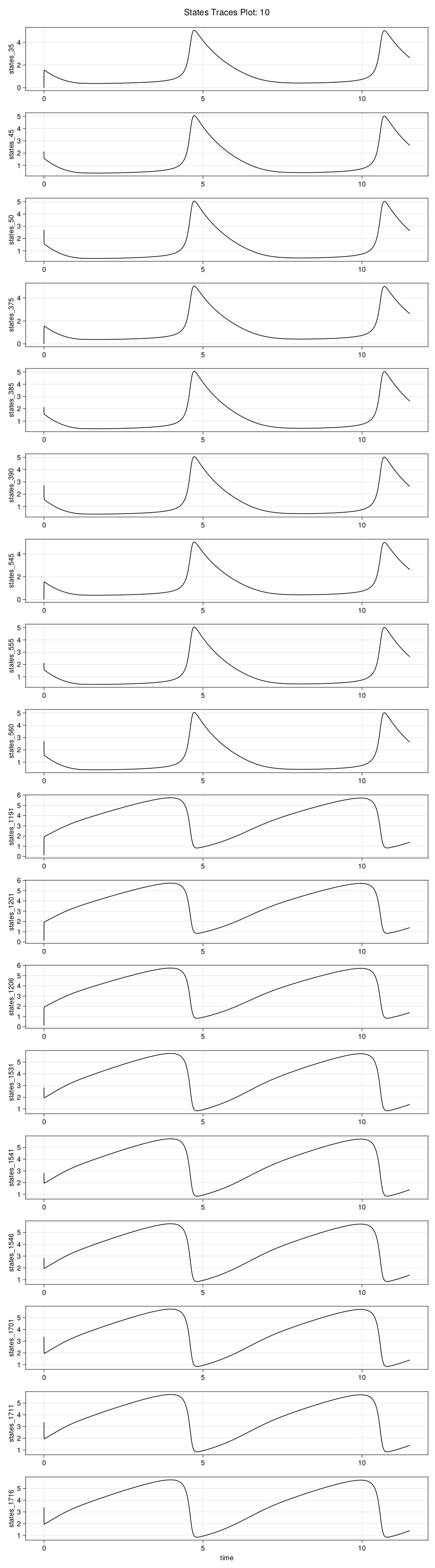
Once we ensure that we have generated data that explores the space sufficiently, we can move on to training a DigitalEcho.
Training DigitalEcho on JuliaHub
Setting up Training Script
We will use @train to write out the training script which will be executed on the job. This is similar to data generation, where we need to write code for both importing the required packages and training a surrogate. Here, we use Surrogatize module to train a DigitalEcho.
@train begin
    using Surrogatize, DataGeneration

    ## Loading the dataset
    dict = JLSO.load(JSS_DATASET_PATH)[:result]
    ed = ExperimentData(dict)

    ## Training
    surrogate = DigitalEcho(ed; tau = 1.0)
end
Deploying the Training Job on JuliaHub
We provide the name of the dataset which will be downloaded for us on the job and the path to it will be stored as JSS_DATASET_PATH. We can reference it in the training script as seen above. We also provide the name of the surrogate dataset where the trained surrogate will be uploaded.
dataset_name = "brusselator"
surrogate_name = "brusselator_digitalecho""brusselator_digitalecho"Next, we provide the specifications of the compute required for the job. As a rule of thumb, we need GPU machines for fitting DigitalEcho for faster training.
training_specs = (ncpu = 8, ngpu = 1, memory = 61, timelimit = 6)(ncpu = 8, ngpu = 1, memory = 61, timelimit = 6)Next, we provide the batch image to use for the job. Again, we will use JuliaSim image as all the packages we need can only be accessed through it.
batch_image = JuliaHub.batchimage("juliasim-batch", "JuliaSim")JuliaHub.BatchImage:
product: juliasim-batch
image: JuliaSim
CPU image: juliajuliasim
GPU image: juliagpujuliasimWe then call run_training to launch and run the job.
train_job, surrogate_dataset = run_training(@__DIR__,
    batch_image,
    dataset_name;
    auth,
    surrogate_name,
    specs = training_specs)
Downloading the Model
Once the training job is finished, we can download the surrogate onto our JuliaSimIDE instance to perform some validations to check whether the surrogate we trained performs well or not.
path_surrogate_dataset = JuliaHub.download_dataset(surrogate_dataset, "local path of the file"; auth)The model is serialized using JLSO, so we deserialize it:
model = JLSO.load(path_surrogate_dataset)[:result]A Continous Time Surrogate wrapper with:
prob:
A `DigitalEchoProblem` with:
model:
A DigitalEcho with :
RSIZE : 256
USIZE : 18
XSIZE : 0
PSIZE : 4
ICSIZE : 0
solver: Tsit5(; stage_limiter! = trivial_limiter!, step_limiter! = trivial_limiter!, thread = static(false),)
Validation of the DigitalEcho
Inference using Training Data
We validate the trained surrogate using one of the training samples.
We get the initial condition, labels for it, parameters and the timesteps to save by indexing into the dataset.
idx = 10
u0 = ed.specs.u0s.vals[idx]
labels = ed.results.states.labels
p = ed.specs.ps.vals[idx]
ts = ed.results.tss.vals[idx]
tspan = ed.specs.tspans.vals[idx]
(0.0, 11.5)We call the forward pass of the surrogate.
pred = model(u0, (u, t) -> nothing, p, tspan; saveat = ts)18×1402 Matrix{Float64}:
-0.000206866 -0.000206866 … 2.76834 2.71345 2.65971 2.62286
2.13569 2.13569 2.76835 2.71351 2.65979 2.62295
2.71642 2.71642 2.76865 2.71382 2.6601 2.62328
-0.000125808 -0.000125808 2.76854 2.71363 2.65989 2.62303
2.13575 2.13575 2.76888 2.71397 2.66021 2.62335
2.71638 2.71638 … 2.77029 2.71531 2.66152 2.62465
-0.000182114 -0.000182114 2.76864 2.71364 2.65984 2.62295
2.13576 2.13576 2.76831 2.71353 2.65984 2.62304
2.71649 2.71649 2.7693 2.7144 2.66065 2.6238
0.135307 0.135307 1.33711 1.35998 1.38298 1.39909
0.1353 0.1353 … 1.33735 1.36012 1.38307 1.39913
0.1353 0.1353 1.33716 1.35999 1.38296 1.39906
2.82843 2.82843 1.33729 1.36012 1.38311 1.39921
2.82838 2.82838 1.33729 1.36015 1.38315 1.39927
2.82833 2.82833 1.33722 1.36009 1.3831 1.39923
3.37049 3.37049 … 1.33711 1.35998 1.38299 1.39912
3.37044 3.37044 1.3371 1.36001 1.38304 1.39919
3.37043 3.37043 1.33722 1.36007 1.38307 1.39919We get the ground truth for the sample.
gt = ed.results.states.vals[idx]18×1402 Matrix{Float64}:
0.0 4.2092e-10 4.20957e-6 … 2.77506 2.72012 2.66613 2.62894
2.13537 2.13537 2.13537 2.77525 2.72031 2.66632 2.62913
2.71598 2.71598 2.71598 2.77559 2.72065 2.66666 2.62947
0.0 4.2092e-10 4.20957e-6 2.77526 2.72033 2.66633 2.62914
2.13537 2.13537 2.13537 2.77564 2.7207 2.66671 2.62952
2.71598 2.71598 2.71598 … 2.77672 2.72178 2.66779 2.6306
0.0 4.2092e-10 4.20957e-6 2.77516 2.72022 2.66623 2.62903
2.13537 2.13537 2.13537 2.77542 2.72048 2.66649 2.6293
2.71598 2.71598 2.71598 2.77598 2.72104 2.66705 2.62985
0.136003 0.136003 0.136006 1.33456 1.35713 1.38001 1.39617
0.136003 0.136003 0.136006 … 1.33456 1.35713 1.38 1.39617
0.136003 0.136003 0.136006 1.33455 1.35713 1.38 1.39617
2.82843 2.82843 2.82843 1.33456 1.35713 1.38 1.39617
2.82843 2.82843 2.82843 1.33455 1.35713 1.38 1.39617
2.82843 2.82843 2.82843 1.33455 1.35712 1.38 1.39616
3.37035 3.37035 3.37035 … 1.33456 1.35713 1.38 1.39617
3.37035 3.37035 3.37035 1.33456 1.35713 1.38 1.39617
3.37035 3.37035 3.37035 1.33455 1.35713 1.38 1.39617Finally, we can plot to compare the prediction and the ground truth.
 plot_traces(
    ts, pred, gt, labels
)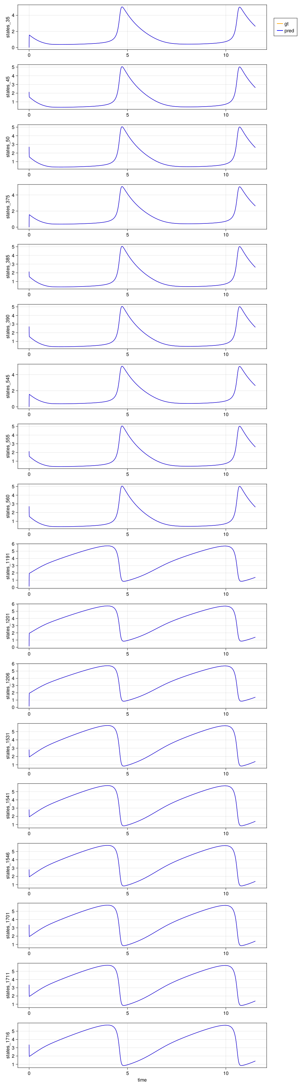
We can see the predictions and ground truth are completely indistinguishable from each other. This is what we say the surrogate has achieved "Line over Line" performance.
Downstream Application: Parameter Estimation
Parameter Estimation is an important procedure in engineering and scientific fields. It is used to determine unknown parameters of a system for a set of observed data by running multiple simulations. Since running multiple simulations is an important part of this procedure, we can leverage the speed we obtain from DigitalEcho.
Evidently, the parameter estimation process using DigitalEcho exhibits significant speed improvement.
Generating an FMU from a DigitalEcho model
We will use @generate_fmu to write out the fmu generation script which will be executed on a separate JuliaHub job. This is important because if you want to generate a windows or linux fmu, you will need a different machine OS to do so. Writing the fmu generation script is similar to what we saw in data generation and training, where we need to write code for both importing the required packages and doing the actual work.
Setting up the FMU generation script
We provide the name of the ExperimentData dataset and the DigitalEcho dataset which will be used in the job and the path to it will be stored as JSS_DATASET_PATH and JSS_MODEL_PATH respectively. We can reference it in the FMU generation script as seen below.
@generate_fmu begin
    using Deployment, JLSO

    ed_dataset = JLSO.load(JSS_DATASET_PATH)[:result]
    ed = ExperimentData(ed_dataset)

    model = JLSO.load(JSS_MODEL_PATH)[:result]

    deploy_fmu(model, ed)
end
Deploying the FMU generation job on JuliaHub
We also provide the name of the FMU dataset where the generated FMU will be uploaded.
dataset_name = "brusselator"
surrogate_name = "brusselator_digitalecho"
fmu_name = "brusselator_fmu""brusselator_fmu"Next, we provide the specifications of the compute required for the job.
fmu_gen_specs = (ncpu = 4, ngpu = 0, memory = 32)(ncpu = 4, ngpu = 0, memory = 32)After that, we provide the batch image to use for the job. Again, we will use JuliaSim image as all the packages we need can only be accessed through it. In this case it will launch a linux machine which will generate a linux based FMU.
batch_image = JuliaHub.batchimage("juliasim-batch", "JuliaSim")JuliaHub.BatchImage:
product: juliasim-batch
image: JuliaSim
CPU image: juliajuliasim
GPU image: juliagpujuliasimWe then call run_fmu_generation to launch and run the job.
job, fmu_dataset = run_fmu_generation(@__DIR__, batchimage, surrogate_name,
    dataset_name;
    fmu_name = fmu_name, auth, specs = fmu_gen_specs, timelimit = 2)
We can choose a Windows Batch Image to generate a Windows based FMU and launch the job as well :
 win_batchimage = JuliaHub.batchimage("winworkstation-batch", "default")

job, win_fmu_dataset = run_fmu_generation(@__DIR__, win_batchimage, surrogate_name,
    dataset_name;
    fmu_name = fmu_name, auth, specs = fmu_gen_specs, timelimit = 2)
With that being done, here is the full script that takes you from data generation to deployment:
######### DataGeneration ##########
@datagen begin
    using Distributed
    addprocs(30, exeflags = ["--project"])

    ## `@everywhere` is used for all the statements which are required in the worker processes for data generation - includes import statements, variables, functions
    @everywhere using OrdinaryDiffEq
    @everywhere using Sundials
    @everywhere using DataGeneration
    using PreProcessing

    ## Defining the function for Brusselator
    @everywhere function brusselator_f(x, y, t)
        (((x - 0.3)^2 + (y - 0.6)^2) <= 0.1^2) * (t >= 1.1) * 5.0
    end
    @everywhere limit(a, N) = a == N + 1 ? 1 : a == 0 ? N : a
    @everywhere function brusselator_2d_loop(u, p, t, xyd_brusselator, N)
        A, B, alpha, dx = p
        du = zeros(size(u)...)
        alpha = alpha / dx^2
        @inbounds for i in 1:N
            iN = (i - 1) * N
            for j in 1:N
                x, y = xyd_brusselator[i], xyd_brusselator[j]
                ip1, im1, jp1, jm1 = limit(i + 1, N),
                limit(i - 1, N),
                limit(j + 1, N),
                limit(j - 1, N)
                idx1 = iN + j
                idx2 = (im1 - 1) * N + j
                idx3 = (ip1 - 1) * N + j
                idx4 = iN + jp1
                idx5 = iN + jm1
                du[idx1] = alpha * (u[idx2] + u[idx3] + u[idx4] + u[idx5] - 4u[idx1]) +
                           B + u[idx1]^2 * u[idx1 + N * N] - (A + 1) * u[idx1] +
                           brusselator_f(x, y, t)
                du[idx1 + N * N] = alpha *
                                   (u[idx2 + N * N] + u[idx3 + N * N] + u[idx4 + N * N] +
                                    u[idx5 + N * N] - 4u[idx1 + N * N]) +
                                   A * u[idx1] - u[idx1]^2 * u[idx1 + N * N]
            end
        end
        du
    end

    ## Defining the function for getting initial state
    @everywhere function init_brusselator_2d(xyd)
        N = length(xyd)
        u = zeros(N * N * 2)
        for i in 1:N
            x = xyd[i]
            for j in 1:N
                y = xyd[j]
                loc = (i - 1) * N + j
                u[loc] = 22 * (y * (1 - y))^(3 / 2)
                u[loc + N * N] = 27 * (x * (1 - x))^(3 / 2)
            end
        end
        u
    end

    ## Discretization of the grid
    @everywhere N = 34
    @everywhere xyd_brusselator = range(0, stop = 1, length = N)
    @everywhere Δx = step(xyd_brusselator)
    @everywhere x_idxs = [1, round(Int, 1 / (3 * Δx)), round(Int, 1 / (2 * Δx))]
    @everywhere y_idxs = N * x_idxs
    @everywhere N_samp = length(x_idxs)

    ## Indices for the selected states
    @everywhere u_idxs = repeat(x_idxs, N_samp, 1)[:] .+ repeat(y_idxs', N_samp, 1)[:]
    @everywhere out_idxs = [u_idxs; N * N .+ u_idxs]

    ## Defining the ODEProblem
    @everywhere u0 = init_brusselator_2d(xyd_brusselator)
    @everywhere tspan = (0.0, 11.5)
    @everywhere p = [3.4, 1.0, 10.0, Δx]
    @everywhere prob = ODEProblem{false}((u, p, t) -> brusselator_2d_loop(u,
            p,
            t,
            xyd_brusselator,
            N),
        u0,
        tspan,
        p)

    ## Defining Parameter Space
    params_lb = [1.7, 0.5, 5.0, Δx - (rand() / 10000)]
    params_ub = [5.1, 1.5, 15.0, Δx + (rand() / 10000)]
    n_samples = 500
    param_space = ParameterSpace(params_lb, params_ub, n_samples)

    ## Setting up SimulatorConfig and generating data
    sim_config = SimulatorConfig(param_space)
    ed = sim_config(prob, verbose = true, abstol = 1e-9, reltol = 1e-9, alg = CVODE_BDF())

    ## Filtering out the selected states from the ExperimentData
    filter = FilterFields(ed, :states, out_idxs)
    filtered_ed = filter(ed)

    ## Converting ExperimentData to a dictionary
    ## This is done such that dictionary form of `ExperimentData` is serialised as it contains only vectors of matrices and strings and no user defined data types
    ed_dict = PreProcessing.convert_ed_to_dict(filtered_ed)
end

batch_image = JuliaHub.batchimage("juliasim-batch", "JuliaSim")
datagen_specs = (ncpu = 32, ngpu = 0, memory = 128, timelimit = 4)
dataset_name = "brusselator"

datagen_job, datagen_dataset = run_datagen(@__DIR__,
   batch_image;
   auth,
   dataset_name,
   specs = datagen_specs)

######### TRAINING ###############
@train begin
    using Surrogatize, DataGeneration

    ## Loading the dataset
    dict = JLSO.load(JSS_DATASET_PATH)[:result]
    ed = ExperimentData(dict)

    ## Training
    surrogate = DigitalEcho(ed; tau = 1.0)
end

surrogate_name = "brusselator_digitalecho"

training_specs = (ncpu = 8, ngpu = 1, memory = 61, timelimit = 6)

train_job, surrogate_dataset = run_training(@__DIR__,
    batch_image,
    dataset_name;
    auth,
    surrogate_name,
    specs = training_specs)

######### FMU GENREATION #############

@generate_fmu begin
    using Deployment, JLSO

    ed_dataset = JLSO.load(JSS_DATASET_PATH)[:result]
    ed = ExperimentData(ed_dataset)

    model = JLSO.load(JSS_MODEL_PATH)[:result]

    deploy_fmu(model, ed)
end
fmu_name = "brusselator_fmu"

fmu_gen_specs = (ncpu = 4, ngpu = 0, memory = 32)

job, fmu_dataset = run_fmu_generation(@__DIR__, batchimage, surrogate_name,
    dataset_name;
    fmu_name = fmu_name, auth, specs = fmu_gen_specs, timelimit = 2)