Running Transient Analysis
Transient analysis solves for the evolution of a circuit's currents and voltages over time. We will showcase here the steps to run a transient analysis, using the circuit from the Butterworth filter example.
Parsing and compiling the SPICE netlist
To parse your SPICE file, pass a file path to the SimManager method. The resultant object represents the parsed and analyzed circuit, and will be used to further create parameterizations and simulations of that circuit. Here we are loading in the butterworth.spice file
using CedarEDA
sm = SimManager("butterworth.spice")
SimManager for 'butterworth.spice', with parameters:
- l1 (default: 1.2n)
- c2 (default: 430p)
- l3 (default: 390n)
- r4 (default: 50)
- freq (default: 10M)CedarEDA features a fully-compiled simulator and will generate specialized machine code to most efficiently simulate this particular circuit, as well as the particular parameterization of this circuit. For this first example, we will create a default parameterization of the circuit via the SimParameterization method. We will tell this particular parameterization to solve over a specific timespan, from 0 to 100 seconds:
# Import some useful suffixes for SI units
using CedarEDA.SIFactors: f, u

sp = SimParameterization(sm; tspan=(0, 1u))
SimParameterization with default parameterization
The SimParameterization object contains within it information about the circuit's signal probe points (sp.probes) which directly correspond to the SPICE file's device and net hierarchy.
julia> sp.probesProbes with 10 properties:
  cc2
  gnd
  ll1
  ll3
  node_0
  node_n1
  node_vin
  node_vout
  rr4
  v1
Running transient simulations
Using this information, we are free to run a transient analysis and visualize the results. The explore method provides a convenient way to visualize analysis results, and if passed a SimParameterization object in isolation, will automatically perform transient analysis. explore() will plot any signals specified as a "saved signal", via the set_saved_signals!() method, which takes in probe points from sp.probes:
# Ensure that `vout` is plotted in `explore()`
set_saved_signals!(sp, [
    sp.probes.node_vout,
])
explore(sp)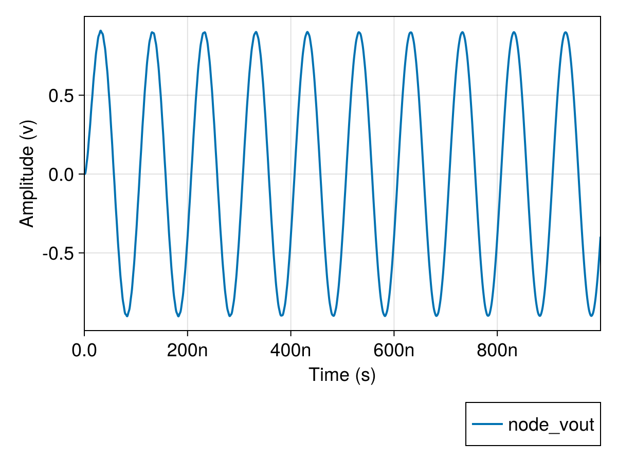
Transient analysis is explicitly requested through tran!(), which returns a SolutionSet object containing the transient signals and convenient syntax for obtaining the signals of interest:
tran_sol = tran!(sp)1-element Transient SolutionTransient solution objects
SolutionSet objects are shaped the same as their originating SimParameterization objects, yielding a natural method of accessing analysis results across parameter sweeps. For an example of using results from a parameter sweep, see Running Parametric Sweeps, but for now we know there is only a single simulation within this transient solution and so will index it by [1] to pull out the first element.
Transient solution objects contain within themselves three properties: op, parameters and tran. The op property is discussed in greater detail in the section on Running DC Analysis, and the parameters property is discussed in Running Parametric Sweeps, and so we will concern ourselves only with the tran property here:
julia> tran_sol.tranTransient Signals with 10 properties:
  cc2
  gnd
  ll1
  ll3
  node_0
  node_n1
  node_vin
  node_vout
  rr4
  v1
The tran property contains within it all signals within the circuit. Critically, one is able to obtain signals that were not listed in set_saved_signals!(), all signals are always available from a solution object, but some may not be saved to .csv when exporting via export_csvs() or plotted via explore().
Signals obtained from SolutionSet objects are CedarWaves signal objects, and can be plotted via the inspect() function. For more information about CedarWaves, view the latest available documentation. Here, we merely show the ease of extracting signals and plotting them, displaying node_vin against node_vout and demonstrating that the filter has indeed decreased the gain. Remember that since our transient analysis contains only a single parameterization point (the default parameterization) we must index our solution signals by [1].
# This will plot both signals within a single figure.
inspect([tran_sol.tran.node_vin[1], tran_sol.tran.node_vout[1]])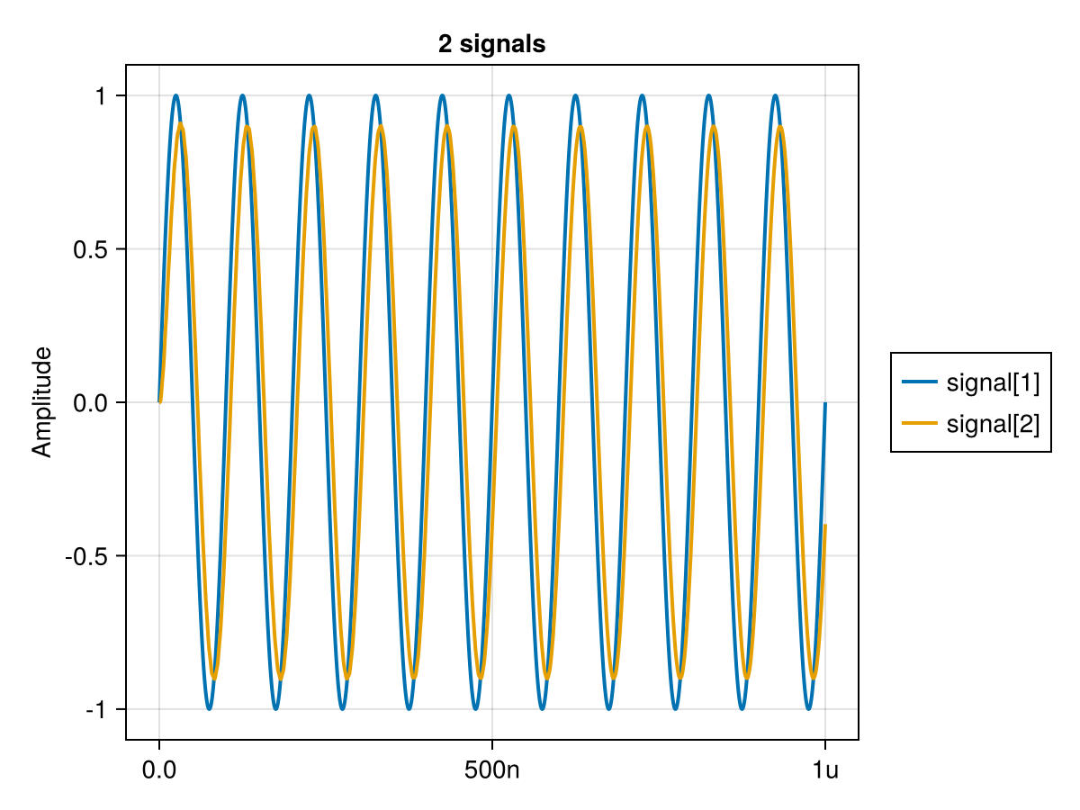
For more on interacting with plots see Working with Plots.
Exporting transient results
To export to .csv, one may use the export_csv() and export_csvs() functions. This is typically used to dump either a specific signal to a single .csv file, or a whole set of simulations to a directory:
# Exporting a single signal as a `.csv`
export_csv("node_vout.csv", tran_sol.tran.node_vout[1])

# Exporting all saved signals, across all parameterization points
export_csvs("outputs", sp)