Running DC Analysis

DC analysis solves for the initial conditions of a circuit's currents and voltages. We will showcase here the steps to run a DC analysis, using the circuit from the Op-Amp Example. If you have not already, we recommend reviewing Running Transient Analysis, and Running Parametric Sweeps as we will be building on top of the concepts covered within.

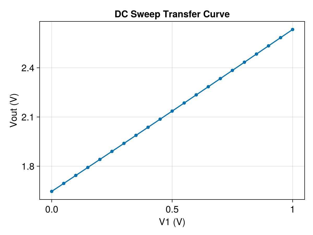
As a first step, we load the SPICE file and prepare a parameterization. We will here sweep parameters setting the input voltage to this op-amp, looking to see the output voltage follow the input voltage, but saturating at some point based on the properties of the amplifier:

using CedarEDA

sm = SimManager(joinpath(@__DIR__, "ota.spice"))
# Sweep `pv1`, and solve the DC operating point to a tight tolerance
dc_sp = SimParameterization(sm;
    params = ProductSweep(;pv1 = 0:0.05:1),
)
dc_sol = dc!(dc_sp)

21-element DC Solution

DC Solution Objects

Just as with a transient analysis solution, a DC analysis solution contains within it a few properties:

julia> dc_sol.parametersParameters with 1 properties:
  pv1

julia> dc_sol.opDC Operating Point with 19 properties:
  cl
  gnd
  node_0
  node_1
  node_2
  node_3
  node_diff_a
  node_ninop
  node_ninp
  node_nmid
  node_nout
  node_second
  node_vdd
  rl
  rq
  v1
  vmid
  vvdd
  x1

Unlike the tran property within a transient solution, the values extracted from the op property are not signals but rather scalar floating point values, one for each point in the parameter sweep:

julia> dc_sol.op.node_nout[1:3]3-element Vector{Float64}:
 1.6465255882705567
 1.6951166575514416
 1.7437794812213296

This, combined with the scalars yielded by the parameters property makes it easy to visualize operating point sweep curves. Here we make use of our inspect() function as before. For more information on plotting in CedarEDA, see Working with Plots.

using WGLMakie

inspect(
    # Create a signal containing operating point against parameter value
    Signal(dc_sol.parameters.pv1, dc_sol.op.node_nout),
    # Override the label names
    xlabel="V1 (V)",
    ylabel="Vout (V)",
    title="DC Sweep Transfer Curve",
)