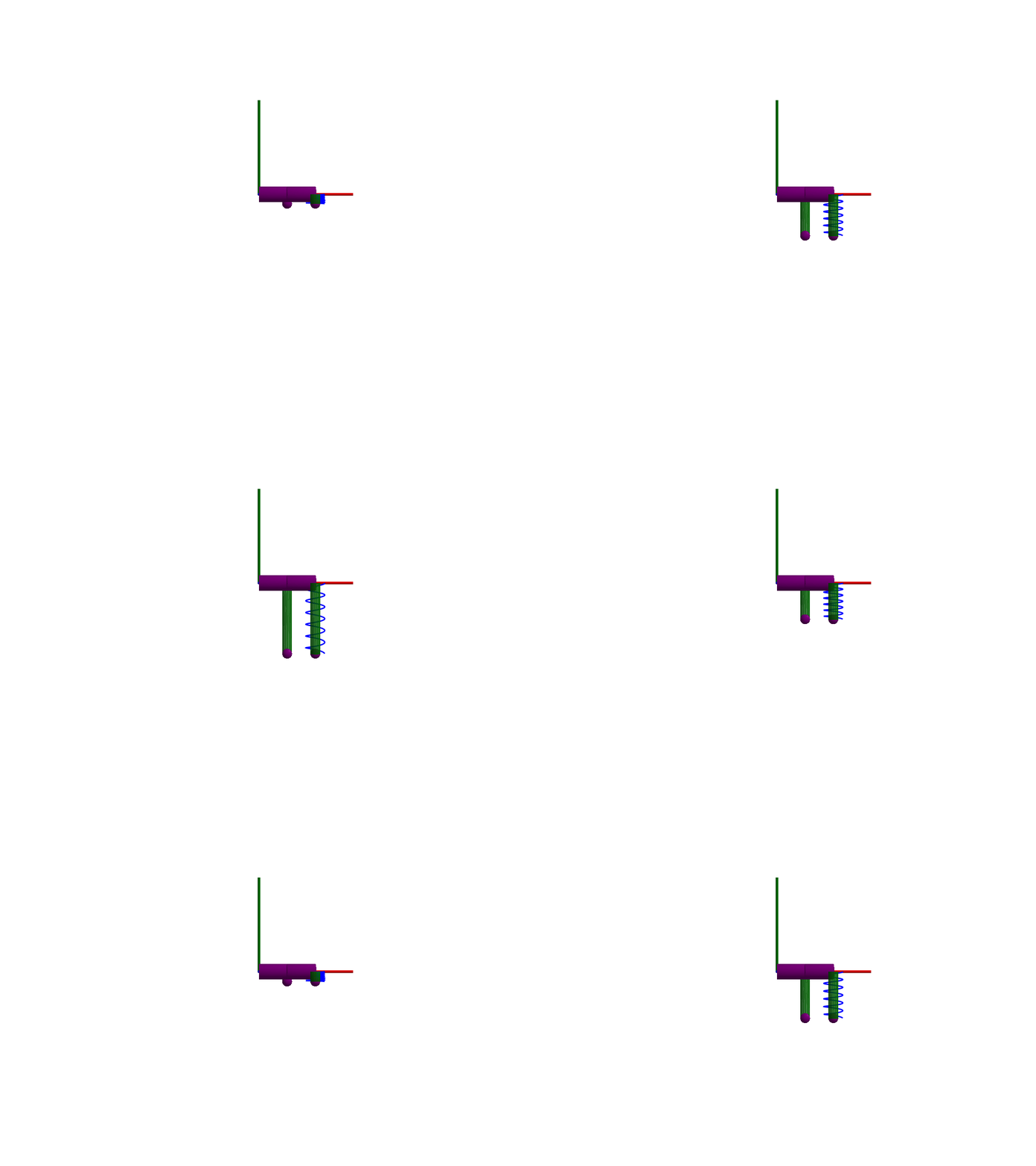
Spring-mass system

This example mirrors that of the modelica spring-mass system and demonstrates that we can model a spring-mass system in two different ways.

1. Using a prismatic joint and a 1-dimensional spring from the Translational submodule attached to the joint. The advantage of this approach is that the many elements from the Translational library can be easily used here and that this implementation is usually more efficient compared to when using 3-dimensional springs.
2. Using a 3-dimensional spring from the Multibody library.

using Multibody
using ModelingToolkit
using Plots
using JuliaSimCompiler
using ModelingToolkitStandardLibrary.Mechanical.TranslationalModelica
using OrdinaryDiffEq

t = Multibody.t
D = Differential(t)
world = Multibody.world

systems = @named begin
    p1      = Prismatic(n = [0, -1, 0], s0 = 0.1, axisflange = true)
    spring1 = TranslationalModelica.Spring(c=30, s_rel0 = 0.1)
    spring2 = Multibody.Spring(c = 30, s_unstretched = 0.1)
    body1   = Body(m = 1, r_cm = [0, 0, 0], radius=0.1, color=[1,0.5,0,1])
    bar1    = FixedTranslation(r = [0.3, 0, 0])
    bar2    = FixedTranslation(r = [0.3, 0, 0])
    body2   = Body(m = 1, r_cm = [0, 0, 0], radius=0.1)
    p2      = Prismatic(n = [0, -1, 0], s0 = 0.1, axisflange = true)
end

eqs = [
    connect(body1.frame_a, p1.frame_b)
    connect(world.frame_b, bar1.frame_a)
    connect(bar1.frame_b, p1.frame_a)
    connect(spring1.flange_b, p1.axis)
    connect(bar1.frame_b, bar2.frame_a)
    connect(bar2.frame_b, p2.frame_a)
    connect(p2.frame_b, body2.frame_a)
    connect(bar2.frame_b, spring2.frame_a)
    connect(body2.frame_a, spring2.frame_b)
    connect(spring1.flange_a, p1.support)
]

@named model = ODESystem(eqs, t, systems = [world; systems])
ssys = structural_simplify(multibody(model))
prob = ODEProblem(ssys,[], (0, 5))

sol = solve(prob, Rodas4())
@assert SciMLBase.successful_retcode(sol)

Plots.plot(sol, idxs = [body1.r_0[2], body2.r_0[2]])

The plot indicates that the two systems behave identically.

3D animation

Multibody.jl supports automatic 3D rendering of mechanisms, we use this feature to illustrate the result of the simulation below:

import GLMakie
Multibody.render(model, sol; x=5, z = 5, filename = "springmass.gif")

You may notice that only one of the springs is rendered, the multibody spring is a 3D mechanical component with a rendering defined, while the spring from the 1D rotational library has no notion of 3D extent.