Free motions

This example demonstrates how a free-floating Body can be simulated. The body is attached to the world through a FreeMotion joint, i.e., a joint that imposes no constraints. The joint is required to add the appropriate relative state variables between the world and the body. We choose state = true and isroot = true in the FreeMotion constructor.

using Multibody
using ModelingToolkit
using Plots
using JuliaSimCompiler
using OrdinaryDiffEq

t = Multibody.t
D = Differential(t)
world = Multibody.world

@named freeMotion = FreeMotion(state = true, isroot = true)
@named body = Body(m = 1)

eqs = [connect(world.frame_b, freeMotion.frame_a)
       connect(freeMotion.frame_b, body.frame_a)]

@named model = ODESystem(eqs, t,
                         systems = [world;
                                    freeMotion;
                                    body])
ssys = structural_simplify(multibody(model))

prob = ODEProblem(ssys, [], (0, 10))

sol = solve(prob, Rodas4())
plot(sol, idxs = body.r_0[2], title="Free falling body")

# Plot analytical solution
tvec = 0:0.1:sol.t[end]
plot!(tvec, -9.81/2 .* tvec .^ 2, lab="Analytical solution")

The figure indicates that the body is falling freely, experiencing a constant acceleration of -9.81 m/s² in the $y$ direction, corresponding to the gravity parameters of the world:

Model world with 19 (25) equations
Unknowns (16):
  (n_inner(t))[1]
  (n_inner(t))[2]
  (n_inner(t))[3]
  g_inner(t)
  mu_inner(t)
  render_inner(t)
  point_gravity_inner(t)
  (frame_b₊r_0(t))[1] [defaults to 0.0]: Position vector directed from the origin of the world frame to the connector frame origin, resolved in world frame
  (frame_b₊r_0(t))[2] [defaults to 0.0]: Position vector directed from the origin of the world frame to the connector frame origin, resolved in world frame
  (frame_b₊r_0(t))[3] [defaults to 0.0]: Position vector directed from the origin of the world frame to the connector frame origin, resolved in world frame
  (frame_b₊f(t))[1]: Cut force resolved in connector frame
  (frame_b₊f(t))[2]: Cut force resolved in connector frame
  (frame_b₊f(t))[3]: Cut force resolved in connector frame
  (frame_b₊tau(t))[1]: Cut torque resolved in connector frame
  (frame_b₊tau(t))[2]: Cut torque resolved in connector frame
  (frame_b₊tau(t))[3]: Cut torque resolved in connector frame
Parameters (10):
  n[1] [defaults to 0.0]: gravity direction
  n[2] [defaults to -1.0]: gravity direction
  n[3] [defaults to 0.0]: gravity direction
  g [defaults to 9.80665]: gravitational acceleration of world
  mu [defaults to 3.986e14]: Gravity field constant [m³/s²] (default = field constant of earth)
  point_gravity [defaults to false]
  render [defaults to true]
  frame_b₊render [defaults to false]
  frame_b₊length [defaults to 1.0]
  frame_b₊radius [defaults to 0.1]

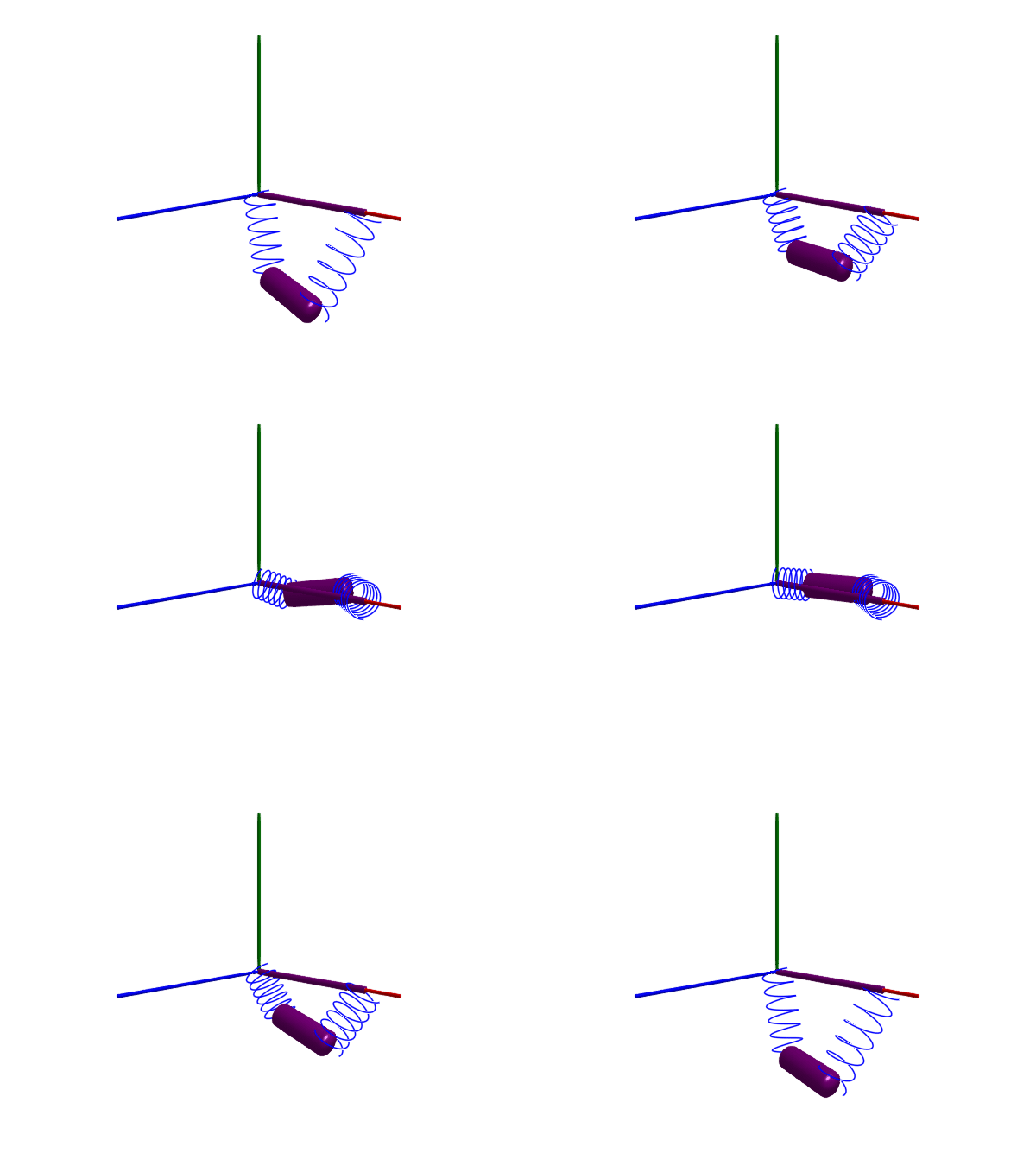
Body suspended in springs

If we instead model a body suspended in springs without the presence of any joint, we need to give the body state variables. We do this by saying isroot = true when we create the body, we also use quaternions to represent angular state using quat = true.

using Multibody.Rotations: QuatRotation, RotXYZ, params
@named begin
    body = BodyShape(m = 1, I_11 = 1, I_22 = 1, I_33 = 1, r = [0.4, 0, 0],
                     r_0 = [0.2, -0.5, 0.1], isroot = true, quat=true)
    bar2 = FixedTranslation(r = [0.8, 0, 0])
    spring1 = Multibody.Spring(c = 20, s_unstretched = 0)
    spring2 = Multibody.Spring(c = 20, s_unstretched = 0)
end

eqs = [connect(bar2.frame_a, world.frame_b)
       connect(spring1.frame_b, body.frame_a)
       connect(bar2.frame_b, spring2.frame_a)
       connect(spring1.frame_a, world.frame_b)
       connect(body.frame_b, spring2.frame_b)]

@named model = ODESystem(eqs, t,
                         systems = [
                             world,
                             body,
                             bar2,
                             spring1,
                             spring2,
                         ])
model = complete(model)
ssys = structural_simplify(multibody(model))
prob = ODEProblem(ssys, [
    collect(body.body.v_0 .=> 0);
    collect(body.body.w_a .=> 0);
    # collect(body.body.phi .=> deg2rad.([10,10,10])); # If using Euler/Cardan angles
    collect(body.body.Q̂) .=> params(QuatRotation(RotXYZ(deg2rad.((10,10,10))...)));
], (0, 4))

sol = solve(prob, Rodas5P())
@assert SciMLBase.successful_retcode(sol)

plot(sol, idxs = [body.r_0...])
# plot(sol, idxs = [body.body.Q...])

import GLMakie
Multibody.render(model, sol, filename = "free_body.gif")