Multibody

Documentation for Multibody.
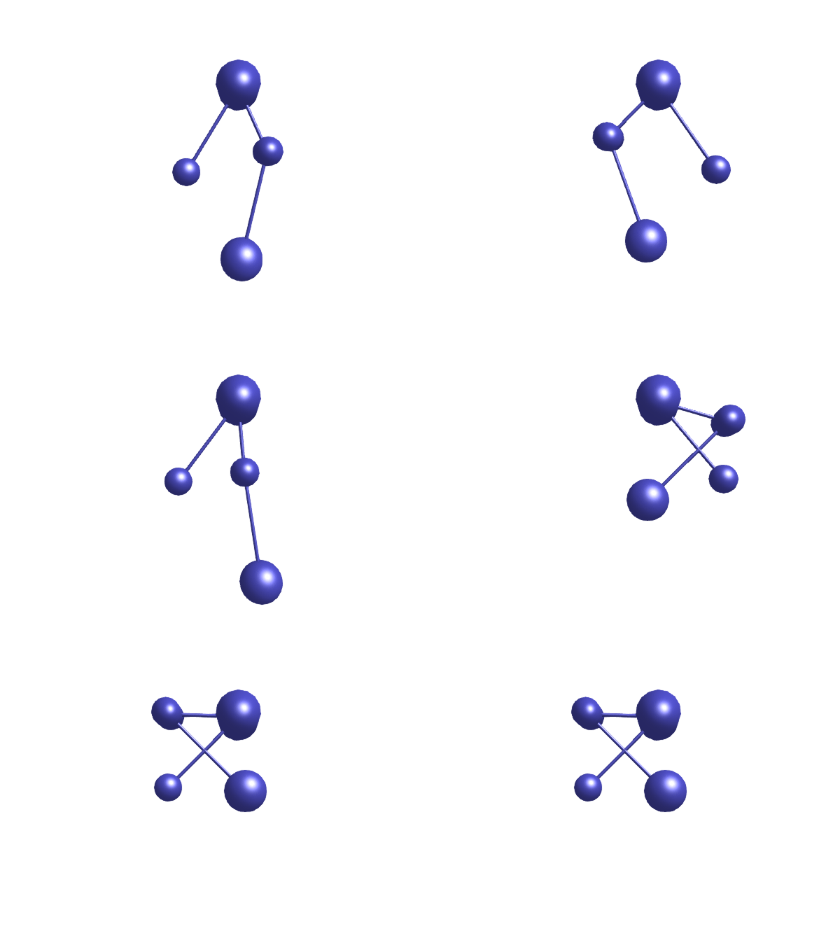
animated logo

Welcome to the world of Multibody.jl, a powerful and flexible component of JuliaSim designed to model, analyze, and simulate multibody systems in Julia. As a state-of-the-art tool, Multibody.jl enables users to efficiently study the dynamics of complex mechanical systems in various fields, such as robotics, biomechanics, aerospace, and vehicle dynamics.

Built on top of the Julia language and the JuliaSim suite of tools for modeling, simulation, optimization and control, Multibody.jl harnesses the power of Julia's high-performance computing capabilities, making it a go-to choice for both researchers and engineers who require fast simulations and real-time performance. With an intuitive syntax and a comprehensive set of features, this package seamlessly integrates with other Julia and JuliaSim libraries, enabling users to tackle diverse and sophisticated problems in multibody dynamics.

In this documentation, you will find everything you need to get started with Multibody.jl, from basic component descriptions to detailed examples showcasing the package's capabilities. As you explore this documentation, you'll learn how to create complex models, work with forces and torques, simulate various types of motions, and visualize your results in both 2D and 3D. Whether you are a seasoned researcher or a newcomer to the field, Multibody.jl will empower you to bring your ideas to life and unlock new possibilities in the fascinating world of multibody dynamics.

Example overview

The following animations give a quick overview of simple mechanisms that can be modeled using Multibody.jl. The examples are ordered from simple at the top, to more advanced at the bottom. Please browse the examples for even more examples!

GIF Grid
Furutaspringdampersphericalthree_springsspacefree_bodyflexible_ropemounted_chainstiff_ropefourbar2fourbarrobot

Notable differences from Modelica

  • The torque variable in Multibody.jl is typically called tau rather than t to not conflict with the often used independent variable t used to denote time.
  • Multibody.jl occasionally requires the user to specify which component should act as the root of the kinematic tree. This only occurs when bodies are connected directly to force components without a joint parallel to the force component.
  • In Multibody.jl, the orientation object of a Frame is accessed using the function ori.
  • Quaternions in Multibody.jl follow the order $[s, i, j, k]$, i.e., scalar/real part first.

Index

Frames

Multibody.FrameFunction
Frame(; name)

Frame is the fundamental 3D connector in the multibody library. Most components have one or several Frame connectors that can be connected together.

The Frame connector has internal variables for

  • r_0: The position vector from the world frame to the frame origin, resolved in the world frame
  • f: The cut force resolved in the connector frame
  • tau: The cut torque resolved in the connector frame
  • Depending on usage, also rotation and rotational velocity variables.
source

Joints

A joint restricts the number of degrees of freedom (DOF) of a body. For example, a free floating body has 6 DOF, but if it is attached to a Revolute joint, the joint restricts all but one rotational degree of freedom (a revolute joint acts like a hinge). Similarily, a Prismatic joint restricts all but one translational degree of freedom (a prismatic joint acts like a slider).

A Spherical joints restricts all translational degrees of freedom, but allows all rotational degrees of freedom. It thus transmits no torque. A Planar joint moves in a plane, i.e., it restricts one translational DOF and two rotational DOF. A Universal joint has two rotational DOF.

Some joints offer the option to add 1-dimensional components to them by providing the keyword axisflange = true. This allows us to add, e.g., springs, dampers, sensors, and actuators to the joint.

Multibody.PlanarConstant
Planar(; n = [0,0,1], n_x = [1,0,0], cylinderlength = 0.1, cylinderdiameter = 0.05, cylindercolor = [1, 0, 1, 1], boxwidth = 0.3*cylinderdiameter, boxheight = boxwidth, boxcolor = [0, 0, 1, 1])

Joint where frame_b can move in a plane and can rotate around an axis orthogonal to the plane. The plane is defined by vector n which is perpendicular to the plane and by vector n_x, which points in the direction of the x-axis of the plane. frame_a and frame_b coincide when s_x=prismatic_x.s=0, s_y=prismatic_y.s=0 and phi=revolute.phi=0.

source
Multibody.FreeMotionMethod
FreeMotion(; name, state = true, sequence, isroot = true, w_rel_a_fixed = false, z_rel_a_fixed = false, phi = 0, phi_d = 0, phi_dd = 0, w_rel_b = 0, r_rel_a = 0, v_rel_a = 0, a_rel_a = 0)

Joint which does not constrain the motion between frame_a and frame_b. Such a joint is only meaningful if the relative distance and orientation between frame_a and frame_b, and their derivatives, shall be used as state.

Note, that bodies such as Body, BodyShape, have potential state variables describing the distance and orientation, and their derivatives, between the world frame and a body fixed frame. Therefore, if these potential state variables are suited, a FreeMotion joint is not needed.

The state of the FreeMotion object consits of:

The relative position vector r_rel_a from the origin of frame_a to the origin of frame_b, resolved in frame_a and the relative velocity v_rel_a of the origin of frame_b with respect to the origin of frame_a, resolved in frame_a (= D(r_rel_a)).

Arguments

  • state: Enforce this joint having state, this is often desired and is the default choice.
  • sequence: Rotation sequence
  • w_rel_a_fixed: = true, if w_rel_a_start are used as initial values, else as guess values
  • z_rel_a_fixed: = true, if z_rel_a_start are used as initial values, else as guess values

Initial condition arguments:

  • phi
  • phi_d
  • phi_dd
  • w_rel_b
  • r_rel_a
  • v_rel_a
  • a_rel_a
source
Multibody.GearConstraintMethod
GearConstraint(; name, ratio, checkTotalPower = false, n_a, n_b, r_a, r_b)

This ideal massless joint provides a gear constraint between frames frame_a and frame_b. The axes of rotation of frame_a and frame_b may be arbitrary.

  • ratio: Gear ratio
  • n_a: Axis of rotation of frame_a
  • n_b: Axis of rotation of frame_b
  • r_a: Vector from frame bearing to frame_a resolved in bearing
  • r_b: Vector from frame bearing to frame_b resolved in bearing
source
Multibody.PrismaticMethod
Prismatic(; name, n = [0, 0, 1], axisflange = false)

Prismatic joint with 1 translational degree-of-freedom

  • n: The axis of motion (unit vector)
  • axisflange: If true, the joint will have two additional frames from Mechanical.Translational, axis and support, between which translational components such as springs and dampers can be connected.

If axisflange, flange connectors for ModelicaStandardLibrary.Mechanics.TranslationalModelica are also available:

  • axis: 1-dim. translational flange that drives the joint
  • support: 1-dim. translational flange of the drive support (assumed to be fixed in the world frame, NOT in the joint)

The function returns an ODESystem representing the prismatic joint.

source
Multibody.RevoluteMethod
Revolute(; name, phi0 = 0, w0 = 0, n, axisflange = false)

Revolute joint with 1 rotational degree-of-freedom

  • phi0: Initial angle
  • w0: Iniitial angular velocity
  • n: The axis of rotation
  • axisflange: If true, the joint will have two additional frames from Mechanical.Rotational, axis and support, between which rotational components such as springs and dampers can be connected.

If axisflange, flange connectors for ModelicaStandardLibrary.Mechanics.Rotational are also available:

  • axis: 1-dim. rotational flange that drives the joint
  • support: 1-dim. rotational flange of the drive support (assumed to be fixed in the world frame, NOT in the joint)

Rendering options

  • radius = 0.05: Radius of the joint in animations
  • length = radius: Length of the joint in animations
  • color: Color of the joint in animations, a vector of length 4 with values between [0, 1] providing RGBA values
source
Multibody.RevolutePlanarLoopConstraintMethod
RevolutePlanarLoopConstraint(; name, n)

Revolute joint that is described by 2 positional constraints for usage in a planar loop (the ambiguous cut-force perpendicular to the loop and the ambiguous cut-torques are set arbitrarily to zero)

Joint where frame_b rotates around axis n which is fixed in frame_a and where this joint is used in a planar loop providing 2 constraint equations on position level.

If a planar loop is present, e.g., consisting of 4 revolute joints where the joint axes are all parallel to each other, then there is no unique mathematical solution if all revolute joints are modelled with Revolute and the symbolic algorithms will fail. The reason is that, e.g., the cut-forces in the revolute joints perpendicular to the planar loop are not uniquely defined when 3-dim. descriptions of revolute joints are used. Usually, an error message will be printed pointing out this situation. In this case, one revolute joint in the loop has to be replaced by model RevolutePlanarLoopCutJoint. The effect is that from the 5 constraints of a 3-dim. revolute joint, 3 constraints are removed and replaced by appropriate known variables (e.g., the force in the direction of the axis of rotation is treated as known with value equal to zero; for standard revolute joints, this force is an unknown quantity).

source
Multibody.RollingWheelMethod
RollingWheel(; name, radius, m, I_axis, I_long, width=0.035, x0, y0, kwargs...)

Ideal rolling wheel on flat surface z=0 (5 positional, 3 velocity degrees of freedom)

A wheel rolling on the x-y plane of the world frame including wheel mass. The rolling contact is considered being ideal, i.e. there is no slip between the wheel and the ground. The wheel can not take off but it can incline toward the ground. The frame frame_a is placed in the wheel center point and rotates with the wheel itself.

Arguments and parameters:

  • name: Name of the rolling wheel component
  • radius: Radius of the wheel
  • m: Mass of the wheel
  • I_axis: Moment of inertia of the wheel along its axis
  • I_long: Moment of inertia of the wheel perpendicular to its axis
  • width: Width of the wheel (default: 0.035)
  • x0: Initial x-position of the wheel axis
  • y0: Initial y-position of the wheel axis
  • kwargs...: Additional keyword arguments passed to the RollingWheelJoint function

Variables:

  • x: x-position of the wheel axis
  • y: y-position of the wheel axis
  • angles: Angles to rotate world-frame into frame_a around z-, y-, x-axis
  • der_angles: Derivatives of angles

Named components:

  • frame_a: Frame for the wheel component
  • rollingWheel: Rolling wheel joint representing the wheel's contact with the road surface
source
Multibody.RollingWheelJointMethod
RollingWheelJoint(; name, radius, angles, x0, y0, z0)

Joint (no mass, no inertia) that describes an ideal rolling wheel (rolling on the plane z=0). See RollingWheel for a realistic wheel model with inertia.

A joint for a wheel rolling on the x-y plane of the world frame. The rolling contact is considered being ideal, i.e. there is no slip between the wheel and the ground. This is simply gained by two non-holonomic constraint equations on velocity level defined for both longitudinal and lateral direction of the wheel. There is also a holonomic constraint equation on position level granting a permanent contact of the wheel to the ground, i.e. the wheel can not take off.

The origin of the frame frame_a is placed in the intersection of the wheel spin axis with the wheel middle plane and rotates with the wheel itself. The y-axis of frame_a is identical with the wheel spin axis, i.e. the wheel rotates about y-axis of frame_a. A wheel body collecting the mass and inertia should be connected to this frame.

Arguments and parameters:

name: Name of the rolling wheel joint component radius: Radius of the wheel angles: Angles to rotate world-frame into frame_a around z-, y-, x-axis

Variables:

  • x: x-position of the wheel axis
  • y: y-position of the wheel axis
  • z: z-position of the wheel axis
  • angles: Angles to rotate world-frame into frame_a around z-, y-, x-axis
  • der_angles: Derivatives of angles
  • r_road_0: Position vector from world frame to contact point on road, resolved in world frame
  • f_wheel_0: Force vector on wheel, resolved in world frame
  • f_n: Contact force acting on wheel in normal direction
  • f_lat: Contact force acting on wheel in lateral direction
  • f_long: Contact force acting on wheel in longitudinal direction
  • err: Absolute value of (r_road_0 - frame_a.r_0) - radius (must be zero; used for checking)
  • e_axis_0: Unit vector along wheel axis, resolved in world frame
  • delta_0: Distance vector from wheel center to contact point
  • e_n_0: Unit vector in normal direction of road at contact point, resolved in world frame
  • e_lat_0: Unit vector in lateral direction of road at contact point, resolved in world frame
  • e_long_0: Unit vector in longitudinal direction of road at contact point, resolved in world frame
  • s: Road surface parameter 1
  • w: Road surface parameter 2
  • e_s_0: Road heading at (s,w), resolved in world frame (unit vector)
  • v_0: Velocity of wheel center, resolved in world frame
  • w_0: Angular velocity of wheel, resolved in world frame
  • vContact_0: Velocity of contact point, resolved in world frame

Connector frames

  • frame_a: Frame for the wheel joint
source
Multibody.SphericalMethod
Spherical(; name, state = false, isroot = true, w_rel_a_fixed = false, z_rel_a_fixed = false, sequence, phi = 0, phi_d = 0, phi_dd = 0, d = 0)

Joint with 3 constraints that define that the origin of frame_a and the origin of frame_b coincide. By default this joint defines only the 3 constraints without any potential state variables. If parameter state is set to true, three states are introduced. The orientation of frame_b is computed by rotating frame_a along the axes defined in parameter vector sequence (default = [1,2,3], i.e., the Cardan angle sequence) around the angles used as state. If angles are used as state there is the slight disadvantage that a singular configuration is present leading to a division by zero.

  • isroot: Indicate that frame_a is the root, otherwise frame_b is the root. Only relevant if state = true.
  • sequence: Rotation sequence
  • d: Viscous damping constant. If d > 0. the joint dissipates energy due to viscous damping according to $τ ~ -d*ω$.

Rendering options

  • radius = 0.1: Radius of the joint in animations
  • color = [1,1,0,1]: Color of the joint in animations, a vector of length 4 with values between [0, 1] providing RGBA values
source
Multibody.UniversalMethod
Universal(; name, n_a, n_b, phi_a = 0, phi_b = 0, w_a = 0, w_b = 0, a_a = 0, a_b = 0, state_priority=10)

Joint where frame_a rotates around axis n_a which is fixed in frame_a and frame_b rotates around axis n_b which is fixed in frame_b. The two frames coincide when revolute_a.phi=0 and revolute_b.phi=0. This joint has the following potential states;

  • The relative angle phi_a = revolute_a.phi [rad] around axis n_a
  • the relative angle phi_b = revolute_b.phi [rad] around axis n_b
  • the relative angular velocity w_a = D(phi_a)
  • the relative angular velocity w_b = D(phi_b)
source

Components

The perhaps most fundamental component is a Body, this component has a single flange, frame_a, which is used to connect the body to other components. This component has a mass, a vector r_cm from frame_a to the center of mass, and a moment of inertia tensor I in the center of mass. The body can be thought of as a point mass with a moment of inertia tensor.

A mass with a shape can be modeled using a BodyShape. The primary difference between a Body and a BodyShape is that the latter has an additional flange, frame_b, which is used to connect the body to other components. The translation between flange_a and flange_b is determined by the vector r. The BodyShape is suitable to model, e.g., cylinders, rods, and boxes.

A rod without a mass (just a translation), is modeled using FixedTranslation.

Multibody.BodyBoxConstant
BodyBox(; name, m = 1, r = [1, 0, 0], r_shape = [0, 0, 0], width_dir = [0,1,0])

Rigid body with box shape. The mass properties of the body (mass, center of mass, inertia tensor) are computed from the box data. Optionally, the box may be hollow. The (outer) box shape is used in the animation, the hollow part is not shown in the animation. The two connector frames frame_a and frame_b are always parallel to each other.

Parameters

  • r: (structural parameter) Vector from frame_a to frame_b resolved in frame_a
  • r_shape: (structural parameter) Vector from frame_a to box origin, resolved in frame_a
  • width_dir: (structural parameter) Vector in width direction of box, resolved in frame_a
  • length_dir: (structural parameter) Vector in length direction of box, resolved in frame_a
  • length: (structural parameter) Length of box
  • width = 0.3length: Width of box
  • height = width: Height of box
  • inner_width: Width of inner box surface (0 <= inner_width <= width)
  • inner_height: Height of inner box surface (0 <= inner_height <= height)
  • density = 7700: Density of cylinder (e.g., steel: 7700 .. 7900, wood : 400 .. 800)
  • color: Color of box in animations
source
Multibody.worldConstant

The world component is the root of all multibody models. It is a fixed frame with a parallel gravitational field and a gravity vector specified by the unit direction world.n (defaults to [0, -1, 0]) and magnitude world.g (defaults to 9.80665).

source
Multibody.AccSensorMethod
AccSensor(;name)

Ideal sensor to measure the absolute flange angular acceleration

Connectors:

  • flange: Flange Flange of shaft from which sensor information shall be measured
  • a: RealOutput Absolute angular acceleration of flange
source
Multibody.AxisControlBusMethod
@connector AxisControlBus(; name)
  • motion_ref(t) = 0: = true, if reference motion is not in rest
  • angle_ref(t) = 0: Reference angle of axis flange
  • angle(t) = 0: Angle of axis flange
  • speed_ref(t) = 0: Reference speed of axis flange
  • speed(t) = 0: Speed of axis flange
  • acceleration_ref(t) = 0: Reference acceleration of axis flange
  • acceleration(t) = 0: Acceleration of axis flange
  • current_ref(t) = 0: Reference current of motor
  • current(t) = 0: Current of motor
  • motorAngle(t) = 0: Angle of motor flange
  • motorSpeed(t) = 0: Speed of motor flange
source
Multibody.BodyMethod
Body(; name, m = 1, r_cm, isroot = false, phi0 = zeros(3), phid0 = zeros(3), r_0=zeros(3))

Representing a body with 3 translational and 3 rotational degrees-of-freedom.

This component has a single frame, frame_a. To represent bodies with more than one frame, see BodyShape, BodyCylinder, BodyBox.

Parameters

  • m: Mass
  • r_cm: Vector from frame_a to center of mass, resolved in frame_a
  • I_11, I_22, I_33, I_21, I_31, I_32: Inertia-matrix elements
  • isroot: Indicate whether this component is the root of the system, useful when there are no joints in the model.
  • phi0: Initial orientation, only applicable if isroot = true and quat = false
  • phid0: Initial angular velocity

Variables

  • r_0: Position vector from origin of world frame to origin of frame_a
  • v_0: Absolute velocity of frame_a, resolved in world frame (= D(r_0))
  • a_0: Absolute acceleration of frame_a resolved in world frame (= D(v_0))

Rendering options

  • radius: Radius of the joint in animations
  • cylinder_radius: Radius of the cylinder from frame to COM in animations (only drawn if r_cm is non-zero). Defaults to radius/2
  • color: Color of the joint in animations, a vector of length 4 with values between [0, 1] providing RGBA values
source
Multibody.BodyShapeMethod
BodyShape(; name, m = 1, r, kwargs...)

The BodyShape component is similar to a Body, but it has two frames and a vector r that describes the translation between them, while the body has a single frame only.

  • r: Vector from frame_a to frame_b resolved in frame_a
  • All kwargs are passed to the internal Body component.
  • shapefile: A path::String to a CAD model that can be imported by MeshIO for 3D rendering. If none is provided, a cylinder shape is rendered.

See also BodyCylinder and BodyBox for body components with predefined shapes and automatically computed inertial properties based on geometry and density.

source
Multibody.FixedRotationMethod
FixedRotation(; name, r, n, sequence, isroot = false, angle)

Fixed translation followed by a fixed rotation of frame_b with respect to frame_a

  • r: Translation vector
  • n: Axis of rotation, resolved in frame_a
  • angle: Angle of rotation around n, given in radians

To obtain an axis-angle representation of any rotation, see Conversion between orientation formats

source
Multibody.RopeMethod
Rope(; name, l = 1, n = 10, m = 1, c = 0, d = 0, kwargs)

Model a rope (string / cable) of length l and mass m.

The rope is modeled as a series of n links, each connected by a Spherical joint. The links are either fixed in length (default, modeled using BodyShape) or flexible, in which case they are modeled as a Translational.Spring and Translational.Damper in parallel with a Prismatic joint with a Body adding mass to the center of the link segment. The flexibility is controlled by the parameters c and d, which are the stiffness and damping coefficients of the spring and damper, respectively. The default values are c = 0 and d = 0, which corresponds to a stiff rope.

  • l: Unstretched length of rope
  • n: Number of links used to model the rope. For accurate approximations to continuously flexible ropes, a large number may be required.
  • m: The total mass of the rope. Each rope segment will have mass m / n.
  • c: The equivalent stiffness of the rope, i.e., the rope will act like a spring with stiffness c.
  • d: The equivalent damping in the stretching direction of the rope, i.e., the taught rope will act like a damper with damping d.
  • d_joint: Viscous damping in the joints between the links. A positive value makes the rope dissipate energy while flexing (as opposed to the damping d which dissipats energy due to stretching).
  • dir: A vector of norm 1 indicating the initial direction of the rope.

Damping

There are three different methods of adding damping to the rope:

  • Damping in the stretching direction of the rope, controlled by the parameter d.
  • Damping in flexing of the rope, modeled as viscous friction in the joints between the links, controlled by the parameter d_joint.
  • Air resistance to the rope moving through the air, controlled by the parameter air_resistance. This damping is quadratic in the velocity ($f_d ~ -||v||v$) of each link relative to the world frame.

Rendering

  • color = [255, 219, 120, 255]./255
  • radius = 0.05f0
  • jointradius=0
  • jointcolor=color
source
Multibody.oriFunction
ori(frame, varw = false)

Get the orientation of sys as a RotationMatrix object.

For frames, the orientation is stored in the metadata field of the system as sys.metadata[:orientation].

If varw = true, the angular velocity variables w of the frame is also included in the RotationMatrix object, otherwise w is derived as the time derivative of R. varw = true is primarily used when selecting a component as root.

source

Forces

Multibody.DamperMethod
Damper(; d, name, kwargs)

Linear damper acting as line force between frame_a and frame_b. A force f is exerted on the origin of frame_b and with opposite sign on the origin of frame_a along the line from the origin of frame_a to the origin of frame_b according to the equation:

\[f = d D(s)\]

where d is the (viscous) damping parameter, s is the distance between the origin of frame_a and the origin of frame_b and D(s) is the time derivative of s.

Arguments:

  • d: Damping coefficient

Rendering

  • radius = 0.1: Radius of damper when rendered
  • length_fraction = 0.2: Fraction of the length of the damper that is rendered
  • color = [0.5, 0.5, 0.5, 1]: Color of the damper when rendered

See also SpringDamperParallel

source
Multibody.ForceMethod
Force(; name, resolve_frame = :frame_b)

Force acting between two frames, defined by 3 input signals and resolved in frame world, frame_a, frame_b (default)

Connectors:

  • frame_a
  • frame_b
  • force: Of type Blocks.RealInput(3). x-, y-, z-coordinates of force resolved in frame defined by resolve_frame.

Keyword arguments:

  • resolve_frame: The frame in which the cut force and cut torque are resolved. Default is :frame_b, options include :frame_a and :world.
source
Multibody.SpringMethod
Spring(; c, name, m = 0, lengthfraction = 0.5, s_unstretched = 0, kwargs)

Linear spring acting as line force between frame_a and frame_b. A force f is exerted on the origin of frame_b and with opposite sign on the origin of frame_a along the line from the origin of frame_a to the origin of frame_b according to the equation:

\[f = c s\]

where c is the spring stiffness parameter, s is the distance between the origin of frame_a and the origin of frame_b.

Optionally, the mass of the spring is taken into account by a point mass located on the line between frame_a and frame_b (default: middle of the line). If the spring mass is zero, the additional equations to handle the mass are removed.

Arguments:

  • c: Spring stiffness
  • m: Mass of the spring (can be zero)
  • lengthfraction: Location of spring mass with respect to frame_a as a fraction of the distance from frame_a to frame_b (=0: at frame_a; =1: at frame_b)
  • s_unstretched: Length of the spring when it is unstretched
  • kwargs: are passed to LineForceWithMass

Rendering

  • num_windings = 6: Number of windings of the coil when rendered
  • color = [0,0,1,1]: Color of the spring when rendered
  • radius = 0.1: Radius of spring when rendered
  • N = 200: Number of points in mesh when rendered. Rendering time can be reduced somewhat by reducing this number.

See also SpringDamperParallel

source
Multibody.SpringDamperParallelMethod
SpringDamperParallel(; name, c, d, s_unstretched)

Linear spring and linear damper in parallel acting as line force between frame_a and frame_b. A force f is exerted on the origin of frame_b and with opposite sign on the origin of frame_a along the line from the origin of frame_a to the origin of frame_b according to the equation:

\[f = c (s - s_{unstretched}) + d \cdot D(s)\]

where c, s_unstretched and d are parameters, s is the distance between the origin of frame_a and the origin of frame_b and D(s) is the time derivative of s.

source
Multibody.TorqueMethod
Torque(; name, resolve_frame = :frame_b)

Torque acting between two frames, defined by 3 input signals and resolved in frame world, frame_a, frame_b (default)

Connectors:

  • frame_a
  • frame_b
  • torque: Of type Blocks.RealInput(3). x-, y-, z-coordinates of torque resolved in frame defined by resolve_frame.

Keyword arguments:

  • resolve_frame: The frame in which the cut force and cut torque are resolved. Default is :frame_b, options include :frame_a and :world.
source

Sensors

A sensor is an object that translates quantities in the mechanical domain into causal signals which can interact with causal components from ModelingToolkitStandardLibrary.Blocks, such as control systems etc.

Multibody.CutForceMethod
BasicCutForce(; name, resolve_frame)

Basic sensor to measure cut force vector. Contains a connector of type Blocks.RealOutput with name force.

  • resolve_frame: The frame in which the cut force and cut torque are resolved. Default is :frame_a, options include :frame_a and :world.
source
Multibody.CutTorqueMethod
CutTorque(; name, resolve_frame)

Basic sensor to measure cut torque vector. Contains a connector of type Blocks.RealOutput with name torque.

  • resolve_frame: The frame in which the cut force and cut torque are resolved. Default is :frame_a, options include :frame_a and :world.
source
Multibody.PartialCutForceBaseSensorMethod
PartialCutForceBaseSensor(; name, resolve_frame = :frame_a)
  • resolve_frame: The frame in which the cut force and cut torque are resolved. Default is :frame_a, options include :frame_a and :world.
source
Multibody.PowerMethod
Power(; name)

A sensor measuring mechanical power transmitted from frame_a to frame_b.

Connectors:

power of type RealOutput.

source

Orientation utilities

Multibody.RotationMatrixType
RotationMatrix

A struct representing a 3D orientation as a rotation matrix.

If ODESystem is called on a RotationMatrix object o, symbolic variables for o.R and o.w are created and the value of o.R is used as the default value for the symbolic R.

Fields:

  • R::R3: The rotation 3×3 matrix ∈ SO(3)
  • w: The angular velocity vector
source
Multibody.NumRotationMatrixMethod
NumRotationMatrix(; R = collect(1.0 * I(3)), w = zeros(3), name, varw = false)

Create a new RotationMatrix struct with symbolic elements. R,w determine default values.

The primary difference between NumRotationMatrix and RotationMatrix is that the NumRotationMatrix constructor is used in the constructor of a Frame in order to introduce the frame variables, whereas RorationMatrix (the struct) only wraps existing variables.

  • varw: If true, w is a variable, otherwise it is derived from the derivative of R as w = get_w(R).

Never call this function directly from a component constructor, instead call f = Frame(); R = ori(f) and add f to the subsystems.

source
Multibody.absolute_rotationMethod
R2 = absolute_rotation(R1, Rrel)
  • R1: Orientation object to rotate frame 0 into frame 1
  • Rrel: Orientation object to rotate frame 1 into frame 2
  • R2: Orientation object to rotate frame 0 into frame 2
source
Multibody.axis_rotationMethod
axis_rotation(sequence, angle; name = :R)

Generate a rotation matrix for a rotation around the specified axis.

  • sequence: The axis to rotate around (1: x-axis, 2: y-axis, 3: z-axis)
  • angle: The angle of rotation (in radians)

Returns a RotationMatrix object.

source
Multibody.connect_orientationMethod
connect_orientation(R1,R2; iscut=false)

Connect two rotation matrices together, optionally introducing a cut joint. A normal connection of two rotation matrices introduces 9 constraints, while a cut connection introduces 3 constraints only. This is useful to open kinematic loops, see Using cut joints (docs page) for an example where this is used.

source
Multibody.get_frameMethod
T_W_F = get_frame(sol, frame, t)

Extract a 4×4 transformation matrix ∈ SE(3) from a solution at time t.

The transformation matrix returned, $T_W^F$, is such that when a homogenous-coordinate vector $p_F$, expressed in the local frame of reference $F$ is multiplied by $T_W^F$ as $Tp$, the resulting vector is $p_W$ expressed in the world frame:

\[p_W = T_W^F p_F\]

See also get_trans and get_rot, Orientations and directions (docs section).

source
Multibody.get_rotMethod
R_W_F = get_rot(sol, frame, t)

Extract a 3×3 rotation matrix ∈ SO(3) from a solution at time t.

The rotation matrix returned, $R_W^F$, is such that when a vector $p_F$ expressed in the local frame of reference $F$ is multiplied by $R_W^F$ as $Rp$, the resulting vector is $p_W$ expressed in the world frame:

\[p_W = R_W^F p_F\]

The columns of $R_W_F$ indicate are the basis vectors of the frame $F$ expressed in the world coordinate frame.

See also get_trans, get_frame, Orientations and directions (docs section).

source
Multibody.get_wMethod
get_w(R)

Compute the angular velocity w from the rotation matrix R and its derivative DR = D.(R).

source
Multibody.resolve1Method
h1 = resolve1(R21, h2)

R12 is a 3x3 matrix that transforms a vector from frame 1 to frame 2. h2 is a vector resolved in frame 2. h1 is the same vector in frame 1.

Typical usage:

resolve1(ori(frame_a), r_ab)
source
Multibody.resolve2Method
h2 = resolve2(R21, h1)

R21 is a 3x3 matrix that transforms a vector from frame 1 to frame 2. h1 is a vector resolved in frame 1. h2 is the same vector in frame 2.

Typical usage:

resolve2(ori(frame_a), a_0 - g_0)
source

Interfaces

Trajectory planning

Two methods of planning trajectories are available

  • point_to_point: Generate a minimum-time point-to-point trajectory with specified start and endpoints, not exceeding specified speed and acceleration limits.
  • traj5: Generate a 5:th order polynomial trajectory with specified start and end points. Additionally allows specification of start and end values for velocity and acceleration.

Components that make use of these trajectory generators is provided:

These both have output connectors of type RealOutput called q, qd, qdd for positions, velocities and accelerations.

See Industrial robot for an example making use of the point_to_point planner.

Multibody.Kinematic5Method
Kinematic5(; time, name, q0 = 0, q1 = 1, qd0 = 0, qd1 = 0, qdd0 = 0, qdd1 = 0)

A component emitting a 5:th order polynomial trajectory created using traj5. traj5 is a simple trajectory planner that plans a 5:th order polynomial trajectory between two points, subject to specified boundary conditions on the position, velocity and acceleration.

Arguments

  • time: Time vector, e.g., 0:0.01:10
  • name: Name of the component

Outputs

  • q: Position
  • qd: Velocity
  • qdd: Acceleration
source
Multibody.KinematicPTPMethod
KinematicPTP(; time, name, q0 = 0, q1 = 1, qd_max=1, qdd_max=1)

A component emitting a trajectory created by the point_to_point trajectory generator.

Arguments

  • time: Time vector, e.g., 0:0.01:10
  • name: Name of the component
  • q0: Initial position
  • q1: Final position
  • qd_max: Maximum velocity
  • qdd_max: Maximum acceleration

Outputs

  • q: Position
  • qd: Velocity
  • qdd: Acceleration

See also Kinematic5.

source
Multibody.traj5Method
q, qd, qdd = traj5(t; q0, q1, q̇0 = zero(q0), q̇1 = zero(q0), q̈0 = zero(q0), q̈1 = zero(q0))

Generate a 5:th order polynomial trajectory with specified end points, vels and accs.

See also point_to_point and Kinematic5.

source
Multibody.point_to_pointMethod
q,qd,qdd,t_end = point_to_point(time; q0 = 0.0, q1 = 1.0, t0 = 0, qd_max = 1, qdd_max = 1)

Generate a minimum-time point-to-point trajectory with specified start and endpoints, not exceeding specified speed and acceleration limits.

The trajectory produced by this function will typically exhibit piecewise constant accleration, piecewise linear velocity and piecewise quadratic position curves.

If a vector of time points is provided, the function returns matrices q,qd,qdd of size (length(time), n_dims). If a scalar time point is provided, the function returns q,qd,qdd as vectors with the specified dimension (same dimension as q0). t_end is the time at which the trajectory will reach the specified end position.

Arguments:

  • time: A scalar or a vector of time points.
  • q0: Initial coordinate, may be a scalar or a vector.
  • q1: End coordinate
  • t0: Tiem at which the motion starts. If time contains time points before t0, the trajectory will stand still at q0 until time reaches t0.
  • qd_max: Maximum allowed speed.
  • qdd_max: Maximum allowed acceleration.

See also KinematicPTP and traj5.

source