Calibration of a Steady State System
In this example, we will demonstrate the usage of SteadyStateExperiment in DyadModelOptimizer. Here, we will consider a ball encountering a drag-force in a viscous medium. From the classical Stoke's Law, assuming a small spherical object falling in a medium, we can describe a linear relationship between drag-force and velocity, where k is defined as a constant, ${6 \pi \eta r v}$, as below:
\[\begin{aligned} F_v &= k*v \\ \end{aligned}\]
Julia Environment
For this example, we will need the following packages:
| Module | Description |
|---|---|
| DyadModelOptimizer | The high-level library used to formulate our problem and perform automated model discovery |
| ModelingToolkit | The symbolic modeling environment |
| OrdinaryDiffEq | The numerical differential equation solvers |
| CSV and DataFrames | We will read our experimental data from .csv files |
| DataSets | We will load our experimental data from datasets on JuliaHub |
| SteadyStateDiffEq | Steady state differential equation solvers |
| Plots | The plotting and visualization library |
using DyadModelOptimizer
using DyadModelOptimizer: get_params
using ModelingToolkit
import ModelingToolkit: D_nounits as D, t_nounits as t
using OrdinaryDiffEq
using CSV, DataFrames
using SteadyStateDiffEq
using Plots
Model setup
In this case, we have considered the effect of two governing forces, the viscous-drag force and the self-weight of the ball, while the ball is travelling through the fluid. Following Newton's 2nd Law of motion in the vertical direction, we can write the following equation:
\[\begin{aligned} \frac{d(v)}{dt} &= g - (b/m)*v \\ \end{aligned}\]
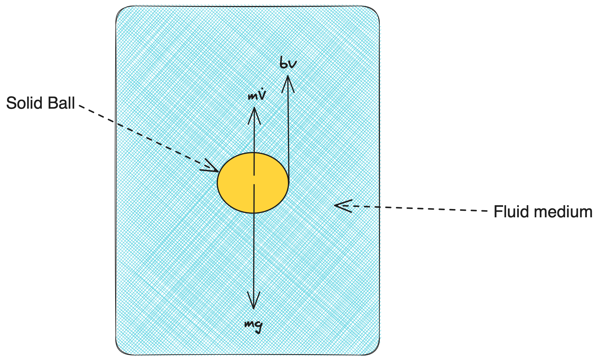
Here, we have two parameters, namely g as the acceleration due to gravity, and k as the constant b/m which takes into account the effect of the viscous drag-force.
@variables v(t)=0
@parameters g=9.8 k=0.2
eqs = [D(v) ~ g - k * v]
@named model = System(eqs, t)
model = complete(model)
\[ \begin{align} \frac{\mathrm{d} v\left( t \right)}{\mathrm{d}t} &= g - k v\left( t \right) \end{align} \]
Data Setup
In order to generate some data, we can simulate a SteadyStateProblem using a steady state solver, here we will use DynamicSS. As our actual data will inherently gather some noise due to measurement error etc, in order to reflect practical scenarios, we have incorporated some Gaussian random noise in our data.
function generate_noisy_data(model; params = [], u0 = [], noise_std = 0.1)
    prob = SteadyStateProblem(model, Dict([u0; params]))
    sol = solve(prob, DynamicSS(Rodas5P()))
    rd = randn(1) * noise_std
    sol.u .+= rd
    return sol
end
data = generate_noisy_data(model, params = [k=>0.3])
retcode: Success
u: 1-element Vector{Float64}:
32.667273461412655Assuming the ball reaches steady-state in Inf secs (which is to signify that it reaches steady-state terminal velocity after a long period of time), we can now create a DataFrame with this timestamp information.
ss_data = DataFrame("timestamp" => Inf, "v(t)" => data.u)| Row | timestamp | v(t) |
|---|---|---|
| Float64 | Float64 | |
| 1 | Inf | 32.6673 |
Defining Experiment and InverseProblem
Once we have generated the data when the ball attains its steady state, we can now create a SteadyStateExperiment for calibration.
experiment = SteadyStateExperiment(ss_data, model; alg = DynamicSS(Rodas5P()))SteadyStateExperiment for model with no overrides.
Once we have created the experiment, the next step is to create an InverseProblem. This inverse problem, requires us to provide the search space as a vector of pairs corresponding to the parameters that we want to recover and the assumption that we have for their respective bounds. Here we will calibrate the value of k, which is usually unknown.
prob = InverseProblem(experiment, [k => (0, 1)])InverseProblem with one experiment with 1 elements in the search space.
Calibration
Now, lets use SingleShooting for calibration. To do this, we first define an algorithm alg and then call calibrate with the prob and alg.
alg = SingleShooting(maxiters = 10^3)
r = calibrate(prob, alg)
Calibration result computed in 19 seconds and 234 milliseconds. Final objective value: 2.29512e-9.
Optimization ended with Success Return Code and returned.
┌──────────┐
│ k │
├──────────┤
│ 0.299994 │
└──────────┘
We can see that the optimizer has converged to a sufficiently small loss value. We can also see that the recovered parameter k matches well with its true value, 0.3!