Performing Global Sensitivity Analysis

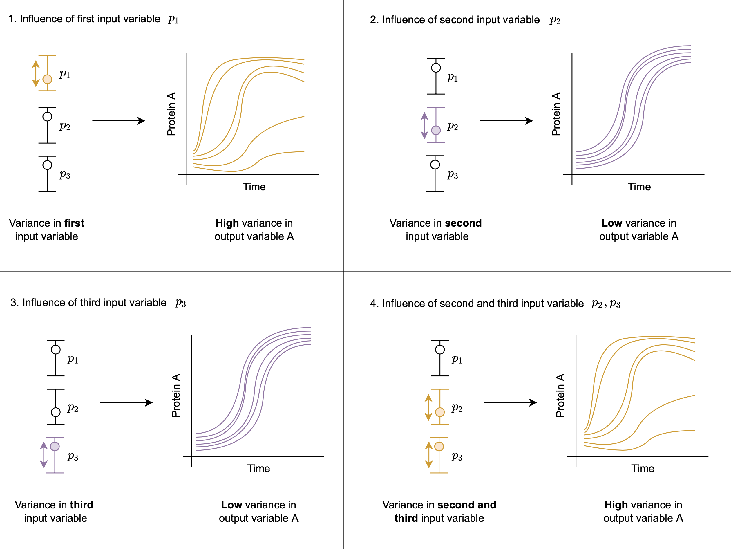
JuliaSimModelOptimizer helps users to consider additional model exploration based on Global Sensitivity Analysis (GSA). This approach is helpful to further investigate how the model output reacts to variance in the model input. For example, we can analyse quantitatively how the variance in single input variables and how combinations of variances in several input variables affect output variables as shown in the figure below:

1. Influence of first input variable,
2. Influence of second input variable,
3. Influence of third input variable,
4. Influence of second and third input variable.

The GlobalSensitivity package provides a large variety of algorithms via gsa(f, method). The function that is used to compuite the sensitivity can be based on simulate, so that one can take advantage of already specified experiments. ^[1]

For example let's consider the predator prey model and perform GSA using the Morris method.

using JuliaSimModelOptimizer
using GlobalSensitivity
using Statistics
using OrdinaryDiffEq
using ModelingToolkit
using Plots
using Test

function lotka()
    @variables t x(t)=3.1 y(t)=1.5
    @parameters α=1.3 β=0.9 γ=0.8 δ=1.8
    ∂ = Differential(t)
    eqs = [
        ∂(x) ~ α * x - β * x * y,
        ∂(y) ~ -δ * y + γ * x * y,
    ]
    @named sys = ODESystem(eqs)
end

sys = complete(lotka())

tspan = (0.0, 10.0)

experiment = Experiment(nothing, sys;
    tspan,
    saveat = range(0, stop = 10, length = 200),
    alg = Tsit5()
)

prob = InverseProblem(experiment, sys,
    [
        sys.α => (1.0, 5.0),
        sys.β => (1.0, 5.0),
        sys.γ => (1.0, 5.0),
        sys.δ => (1.0, 5.0),
    ])

function f(x)
    sol = simulate(experiment, prob, x)
    [mean(sol[:x]), maximum(sol[:y])]
end

lb = lowerbound(prob)
ub = upperbound(prob)

param_range = [[l, u] for (l, u) in zip(lb, ub)]

m = gsa(f, Morris(total_num_trajectory=1000, num_trajectory=150), param_range)

GlobalSensitivity.MorrisResult{Matrix{Float64}, Vector{Any}}([0.004543523855983178 -0.018111287558474926 -0.5139740190237378 0.3706877884096759; 0.6406624983575802 -2.2381618155720817 1.0563826092372333 -0.6196753236106077], [0.1900803783401317 0.03949743691319286 0.5139740190237378 0.37071238181914307; 0.6495027908253749 2.2412709671878126 1.0849994719727607 0.6423357810407998], [0.10225833870845862 0.003589392075786702 0.3684825208001061 0.12684170312866028; 0.6867624424045052 15.365709757198506 0.6139521586551419 0.478979957981294], Any[[[-0.4214000059887956, -0.0277333024616218], [-0.44040406925928116, 0.011441725691324272], [-0.4325653049795494, 0.041147996824692404], [-0.12485524657391858, 0.23536897751453237], [-0.10730269902922243, 0.23228419458201316], [0.1500215007631079, 0.15728157243443186], [0.1274590242055656, 0.12842454562101774], [0.20458831250939033, 0.08154841876796484], [0.07211820717446486, 2.3009807043405894], [-0.08184861646814179, 0.6843358190838651]  …  [-0.13834099427018484, 0.0796434563303999], [-0.1617299127114957, 0.04857651234385685], [-0.11264644006713936, 0.12142721047940436], [0.024544434777483727, 0.2948620018923672], [0.41729421419142865, -0.09538624120531634], [2.1684745413142665, 0.061753875311340974], [-0.07378661786194671, 0.5000627810172599], [-0.07378661786194671, 0.5000627810172599], [-0.0658029882215317, 0.5496718170713257], [-0.35812234532915305, 0.1514178964730232]], [[0.07701092565912027, -0.057128931277785476], [0.02128009650003535, -0.5154170984117263], [-0.01871717210707179, -0.23819135401781702], [-0.01871717210707179, -0.23819135401781702], [-0.01871717210707179, -0.23819135401781702], [-0.018130331987884933, -0.24472715792620167], [-0.03786017811833856, -0.2293420044200791], [0.0009425276008372891, -0.2730280313986094], [-0.02451854411971028, -0.29214259054974123], [0.06967718139849209, -9.81857790997772]  …  [-0.016889238726356757, -1.777679997459362], [-0.016889238726356757, -1.777679997459362], [-0.2509947610247639, 0.014341885440310806], [-0.2528847593748576, -0.10819504874997374], [-0.2528847593748576, -0.10819504874997374], [-0.28848541797644456, -0.014648233722914367], [-0.03342045528572352, -1.2028055207221457], [0.03003147351521637, -0.27477998729479997], [0.03224437009793305, -0.2683508302714712], [0.053420793334409064, -0.2796798383929092]], [[-0.6870232701210675, 0.3272223942590438], [-0.7230630248517361, 0.3034393879836784], [-0.7230630248517361, 0.3034393879836784], [-0.18875317104055594, 0.6701482559942646], [-0.1848681656436156, 0.6706050403328845], [-0.5744860524612485, 0.6074785809960737], [-0.7276525614728714, 0.6090446392721277], [-0.7926787103253855, 1.9391381716846543], [-0.7655741160177382, 1.8969743990522896], [-0.7655741160177382, 1.8969743990522896]  …  [-0.40070945972864164, 2.0215569955365673], [-0.8656297626672055, 0.2348379097150187], [-0.8578759757438328, 0.27678785869062267], [-0.9466237231872213, 0.4960668592548563], [-0.9454346298045293, 0.24776138947144424], [-0.7401373892691699, 1.215647614100063], [-0.6938098747714101, 1.212234016484996], [-0.3647990122381007, 0.6253107825875704], [-0.3655807460475338, 0.6152905169910201], [-0.3658264284538394, 0.6267319322792507]], [[0.20473358020429552, -0.158609661455435], [0.20039036385729986, -0.15789356931488283], [0.10007308960901859, -0.34112043207852527], [0.10007308960901859, -0.34112043207852527], [0.08143236654244188, -0.33910668850552855], [0.08143236654244188, -0.33910668850552855], [0.4831573104327588, -0.2062495271804674], [0.39013817216264596, -0.23907089732668088], [0.5712974384522526, -0.40656979456659176], [0.6153804855812984, -0.2600676415922344]  …  [0.39639810708542134, -0.2599846291133585], [0.44746136792145197, -0.12688964353019597], [0.30790235193669213, -0.61271782001342], [0.48384231160286933, -0.27700412367064836], [1.2426433780079995, -0.8373463275618962], [0.32290897335177415, -0.5369565076838029], [0.3258652041302627, -0.4953450421946827], [0.3258652041302627, -0.4953450421946827], [0.146397904116692, -0.28149218550981986], [0.14565318540892513, -0.2829020673670945]]])

We can plot the results using

scatter(m.means[1,:], m.variances[1,:], series_annotations=[:α,:β,:y,:δ], color=:gray)

and

scatter(m.means[2,:], m.variances[2,:], series_annotations=[:α,:β,:y,:δ], color=:gray)

For the Sobol method, we can similarly do:

m = gsa(f, Sobol(), param_range, samples=1000)

GlobalSensitivity.SobolResult{Matrix{Float64}, Nothing, Nothing, Nothing}([-0.0008389428883520519 -8.756670289610017e-5 0.5453477447320645 0.35422274149024063; 0.06407858586209089 0.5004449209741907 0.23566374011216046 0.0656586576659527], nothing, nothing, nothing, [0.00626573037556132 0.003431279478512331 0.6315860428169109 0.4426612886457248; 0.13079977909017643 0.6194845252432749 0.2860124582905267 0.09457763813881277], nothing)

See the documentation for GlobalSensitivity for more details.