Parametric uncertainty quantification
In DyadModelOptimizer one can perform parametric uncertainty quantification using parametric_uq with an InverseProblem. The result of a parametric_uq call is a set of parameters which sufficiently fit all experiments to their respective data simultaneously. We refer to this as the ensemble of plausible parameters.
The parametric_uq Function
DyadModelOptimizer.parametric_uq — Functionparametric_uq(prob, alg; sample_size, adtype = Optimization.AutoForwardDiff(), progress = true)Create an ensemble of the given size of possible solutions for the inverse problem using the method specified by alg. This can be seen as a representation of the parametric uncertainty characterizing the given inverse problem. This is also called a multimodel in some domains.
Arguments
prob: anInverseProblemobject.alg: a parametric uncertainty quantification algorithm, e.g.StochGlobalOpt. This can beJuliaHubJobfor launching batch jobs in JuliaHub. In this case, the actualalgis wrapped insideJuliaHubJobobject.
Keyword Arguments
sample_size: Required. Number of samples to generate.adtype: Automatic differentiation choice, see the Optimization.jl docs for details. Defaults toAutoForwardDiff().progress: Show the progress of the optimization (current loss value) in a progress bar. Defaults totrue.
Stochastic Optimization
If alg is a StochGlobalOpt method, the optimization algorithm runs until convergence or until maxiters has been reached. This process is repeated a number of times equal to sample_size to create an ensemble of possible parametrizations.
Optimization Methods
The following are the choices of algorithms which are available for controlling the parametric uncertainty quantification process:
DyadModelOptimizer.StochGlobalOpt — TypeStochGlobalOpt(; method = SingleShooting(optimizer = BBO_adaptive_de_rand_1_bin_radiuslimited(), maxiters = 10_000), parallel_type = EnsembleSerial())A stochastic global optimization method.
Keyword Arguments
parallel_type: Choice of parallelism. Defaults toEnsembleSerial()or serial computation. For more information on ensemble parallelism types, see the ensemble types from SciMLmethod: a calibration algorithm to use during the runs. Defaults toSingleShooting(optimizer = BBO_adaptive_de_rand_1_bin_radiuslimited(), maxiters = 10_000). i.e. single shooting method with a black-box differential evolution method from BlackBoxOptimization. For more information on choosing optimizers, see Optimization.jl.
Result Types
DyadModelOptimizer.ParameterEnsemble — TypeParameterEnsembleThe structure contains the result of a parameter ensemble when a StochGlobalOpt method was used to generate the population. To export results to a DataFrame use DataFrame(ps) and to plot them use plot(ps, experiment), where ps is the ParameterEnsemble and experiment is the AbstractExperiment, whose default parameter (or initial condition) values will be used.
Importing Parameter ensembles
If an ensemble of parameters was generated in some alternative way, DyadModelOptimizer still allows for importing these values into a ParameterEnsemble to enable using the parametric uncertainty quantification analysis workflow. This is done via the following function:
DyadModelOptimizer.import_ps — Functionimport_ps(ps, prob)Import a ParameterEnsemble object (ParameterEnsemble) from tabular data.
Arguments
ps: tabular data that contains the parameters of the population. This could be e.g aDataFrameor aCSV.File.prob: anInverseProblemobject.
Analyzing Parameter Ensemble Results
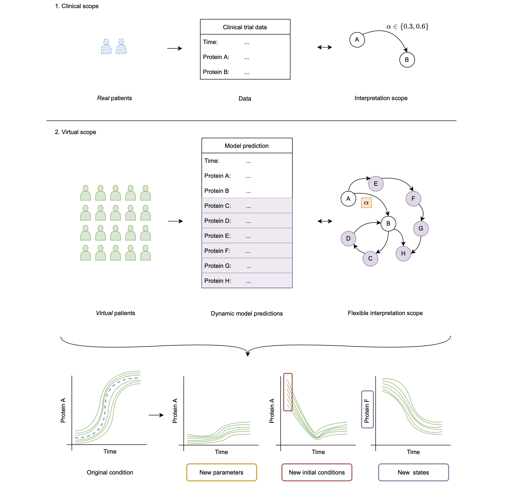
Once parameters (PS) are generated given some multi-experiment data, we can use them to expand our analysis scope to dimensions where, for example, experimental data collection is difficult. This objective is schematically shown in the figure below. Here, we summarise three groups:
- We can use the PS to model the system for new values of model parameters. Note that here we refer to model parameters not as parameters that specify a patient, but other, independent parameters of the model. As an example we have the reaction rate α.
- We can use the PS to model the system for new initial conditions for the observed states of the system. Here, this relates to Protein A and B.
- We can use the PS to model states of the system that have not been observed. These are Protein C to H in this example.
The following functions enable such analyses:
DyadModelOptimizer.solve_ensemble — Functionsolve_ensemble(ps, experiment)Create and solve an EnsembleProblem descrbing the parameters in the ensemble ps and using experiment for the parameter and initial condition values.
Positional Arguments
ps: Object obtained from doingparametric_uq.experiment:Experimentdefined for the Inverse Problem.