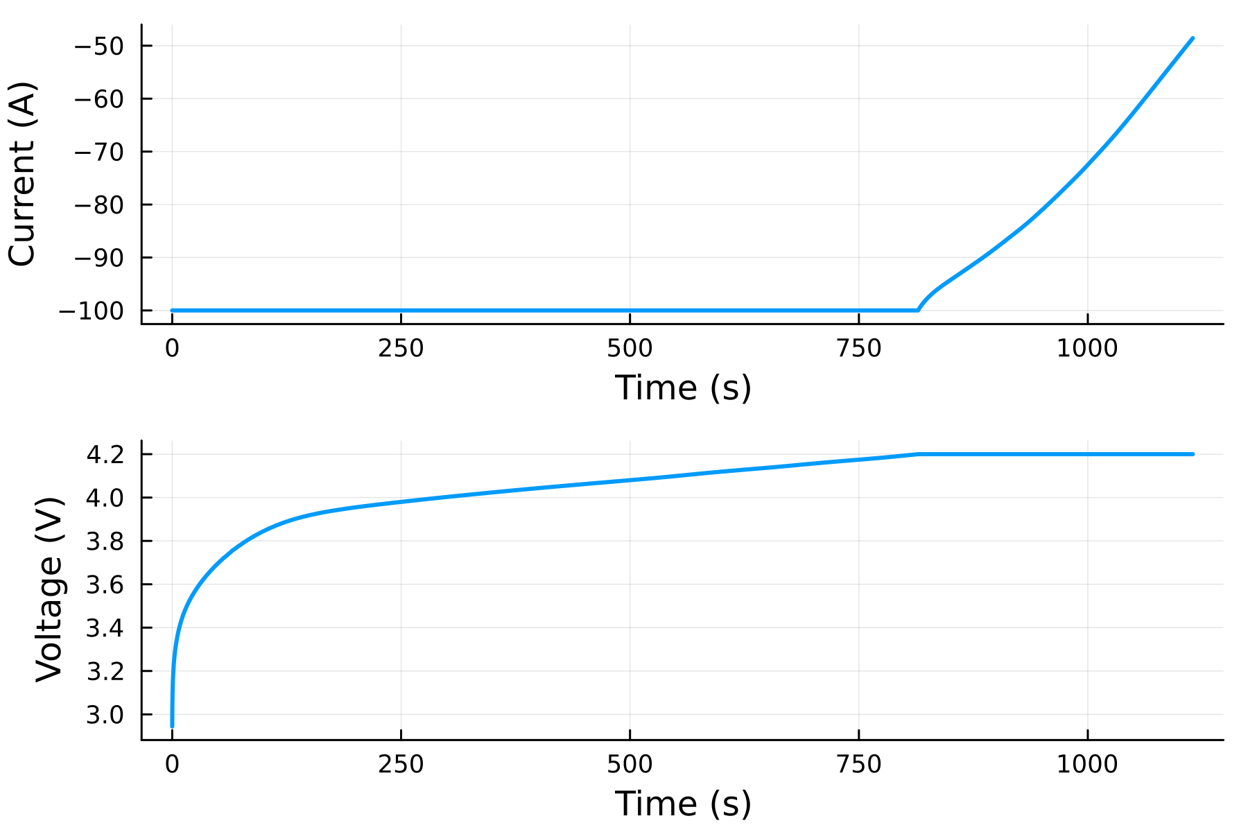
Multi-step charge

Oftentimes, we want to run a series of consecutive experiments on a battery. For example, we may want to charge a battery at a constant current until it reaches a certain voltage, then hold it at that voltage. We can do this by passing in a vector of experiments to the solve function. Here, we charge the battery at 100 A until it reaches 4.2 V, then hold it at that voltage for 300 seconds.

using JuliaSimBatteries, Plots

cell = DFN(LCO())

experiments = [
  charge(100; bounds = "pack voltage maximum" => 4.2)
  voltage(4.2; time = 300)
]

sol = solve(cell, experiments; SOC_initial = 0)

plot(
  plot(sol, "current"),
  plot(sol, "voltage"),
  layout = (:, 1), width = 3, size = (600, 400), dpi = 300
)

By convention, charging is denoted by currents with a negative sign and discharging with a positive sign. The voltage function takes a keyword argument time that specifies how long to hold the voltage at the specified value, or until a constraint is activated.

A list of available experiments is given below. The first input to the current and power functions must have the correct sign for the experiment. For example, if we want to discharge at 100 A. If the unit is not specified, the default unit is the SI base unit. Rest does not take an input, but the time must be specified using the keyword argument time.

• charge
• discharge
• voltage
• rest
• power
• current

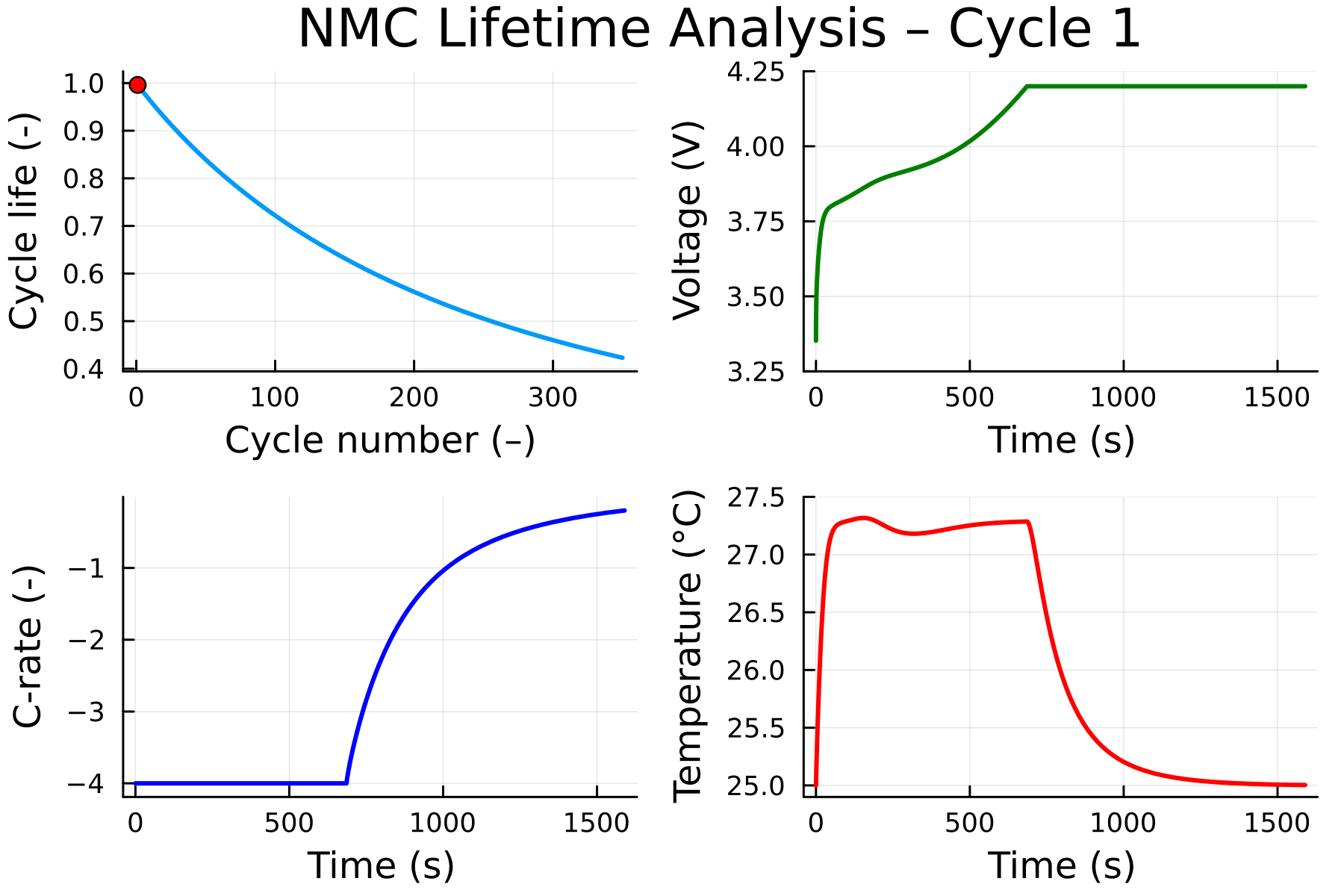
Lifetime simulation

We can also run a series of experiments to simulate multiple charge and discharge cycles. A discharge cycle is added to the experiments array of the previous example with 1 hour intermittent rest periods. The repeat function is used to repeat the experiments for 350 cycles.

using JuliaSimBatteries, Plots, Unitful

cell = DFN(LCO())

# Set the heat transfer coefficients at the current collectors
setparameters(cell, (
    "ambient_1 heat_transfer_coefficient" => 1,
    "ambient_2 heat_transfer_coefficient" => 1,
))

# Disable the bounds on the state of charge
setbounds(cell, (
    "pack state of charge minimum" => NaN,
    "pack state of charge maximum" => NaN,
))

one_cycle = [
  # CC-CV charge
  charge(4C)
  voltage(hold)
  # rest
  rest(time = 3600)
  # C/2 discharge
  discharge(C/2)
  # rest
  rest(time = 3600)
]

cycle_count = 350

experiments = repeat(one_cycle, cycle_count)

sol = solve(cell, experiments, SOC_initial = 0)

soh_cycle = sol["state of health"][last.(cycle_indices(sol))]

tspan = (0, sol.t[cycle_indices(sol; charge=true)[1][end]] / 3600)

@gif for cycle in 1:cycle_count
    kwargs = (; cycle=cycle, charge=true, time_unit=u"hr", xlims=tspan,
              width=3, legend=false, xwiden=1.06, ywiden=1.06)

    ## State of Health
    plt1 = plot(1:cycle, 100(soh_cycle)[1:cycle];
                xlabel = "cycle number (–)", ylabel="state of health (%)", kwargs...)
    scatter!(plt1, [cycle], [100(soh_cycle)[cycle]]; color = :red)
    xlims!(plt1, (1, cycle_count))
    ylims!(plt1, 100 .*(soh_cycle[end], 1))

    plt2 = plot(sol, "voltage";
                color = :green, kwargs...)
    
    plt3 = plot(sol, "C-rate";
                kwargs...)
    ylims!(plt3, (-4, 0))
    
    plt4 = plot(sol, "cell-averaged temperature";
                unit=u"°C", color = :red, kwargs...)

    plot(plt1, plt2, plt3, plt4)
end