Getting Started
This guide describes how to get started using pre-built models and chemistries from JuliaSimBatteries.jl.
To use JuliaSimBatteries, follow the instructions on setting up the JuliaSim IDE on the JuliaHub Cloud platform. JuliaSimBatteries is unavailable for local installation through the JuliaHub registry.
Creating a battery
The first step is to generate a cell. We can use the pseudo-2D Doyle-Fuller-Newman model by evaluating DFN with the desired chemistry. Here, we use the lithium cobalt oxide (LCO) chemistry.
using JuliaSimBatteries

cell = DFN(LCO())
Multiple cathode chemistries are available, including
LCO(lithium cobalt oxide)NMC(lithium nickel manganese cobalt oxide)NCA(lithium nickel cobalt aluminum oxide)LFP(lithium iron phosphate)
Packs and modules
A battery pack is created by connecting multiple batteries in series and parallel. To create a pack, we can use the connection keyword argument to the DFN function. Here, we create a pack with 2 cells in series and 3 cells in parallel.
pack = DFN(LCO(); connection = Pack(series = 2, parallel = 3))Simple discharge experiment
To run a simple experiment on the cell, we can use the solve function. The first argument is cell created above, and the second argument is the type of experiment we want to run. Here, we run a discharge experiment at a C-rate of 1C. C-rate is a measure of the current relative to the capacity of the battery, where 1C fully discharges a battery in 60 minutes and a C-rate of 2C fully discharges a battery in 30 minutes. A default initial state of charge (SOC) is given in the function for the LCO chemistry, and we can override that by passing in a value for SOC_initial.
sol = solve(cell, discharge(1C); SOC_initial = 1)The output of the simulation sol contains the time series of the states of the battery. We can plot the voltage of the battery using the plot function. We can access the states by indexing sol, such as
sol["voltage"]The available states can be accessed by evaluating getstates on the cell
getstates(cell)and plotted using the Plots package
using Plots
plot(sol, "voltage")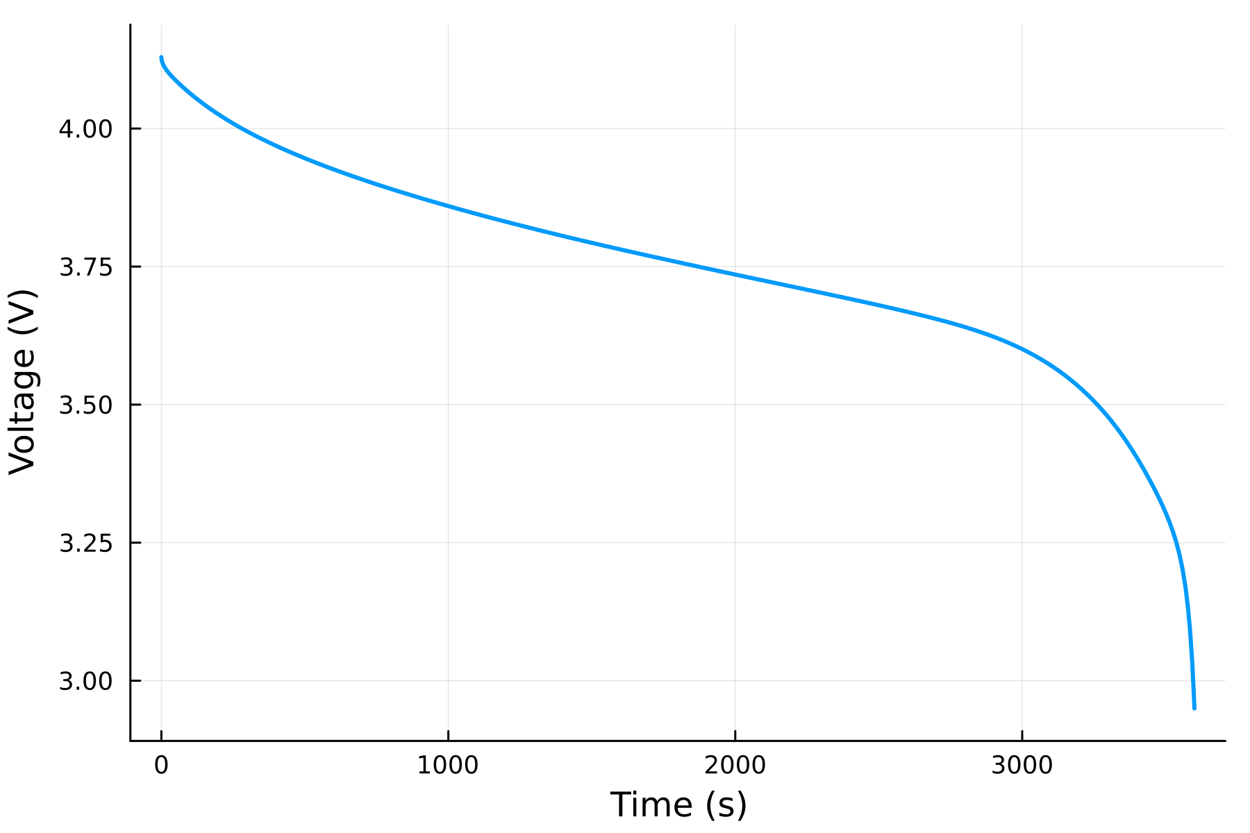
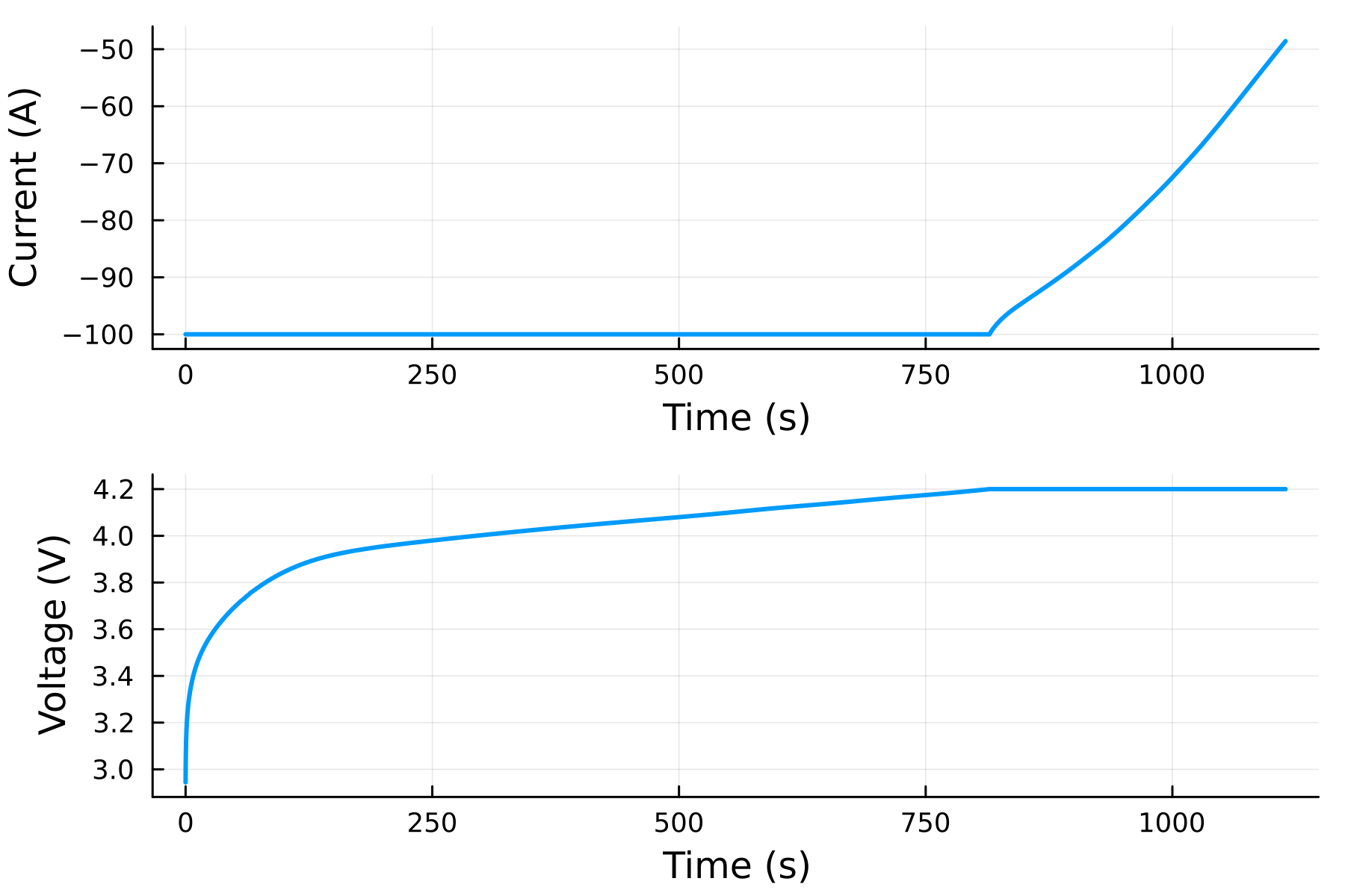
Multi-step charge
Oftentimes, we want to run a series of consecutive experiments on a battery. For example, we may want to charge a battery at a constant current until it reaches a certain voltage, then hold it at that voltage. We can do this by passing in a vector of experiments to the solve function. Here, we charge the battery at 100 A until it reaches 4.2 V, then hold it at that voltage for 300 seconds.
experiments = [
  charge(100; bounds = "pack voltage maximum" => 4.2)
  voltage(4.2; time = 300)
]

sol = solve(cell, experiments; SOC_initial = 0)

plot(
  plot(sol, "current"),
  plot(sol, "voltage"),
  layout = (:, 1)
)
By convention, charging is denoted by currents with a negative sign and discharging with a positive sign. The voltage function takes a keyword argument time that specifies how long to hold the voltage at the specified value, or until a constraint is activated.
A list of available experiments is given below. The first input to the current and power functions must have the correct sign for the experiment. For example, if we want to discharge at 100 A. If the unit is not specified, the default unit is the SI base unit. Rest does not take an input, but the time must be specified using the keyword argument time.
Lifetime simulation
We can also run a series of experiments to simulate multiple charge and discharge cycles. A discharge cycle is added to the experiments array of the previous example with 1 hour intermittent rest periods. The repeat function is used to repeat the experiments for 350 cycles. Let's change the chemistry to NMC and run the lifetime analysis:
using JuliaSimBatteries, Plots, Unitful

cell = DFN(NMC())

# Disable the bounds on the state of charge
disablebounds(cell, ("pack state of charge minimum", "pack state of charge maximum"))

one_cycle = [
  # C/2 discharge
  discharge(C/2)
  # rest
  rest(time = 3600)
  # CC-CV charge
  charge(4C)
  voltage(:hold)
  # rest
  rest(time = 3600)
]

cycle_count = 350

experiments = repeat(one_cycle, cycle_count)

sol = solve(cell, experiments, SOC_initial = 1)
JuliaSimBatteries
-----------------
Runs: 3 I → V → 4 I → …1736… → 4 I → V → I
Time: 54.05 days (350 cycles)
Current: 0.0 A (0C)
Voltage: 4.1704 V
Temp.: 25.0°C
Power: 0.0 W
SOC: 46.0%
Exit: Stop time reachedIn a matter of seconds, we can simulate the full lifetime of a cell. We can visualize the lifetime analysis using an animation for a few keys states of the cell during fast-charge.
function plot_cycle(sol, cycle)
  sol_cycle = sol(; cycle = cycle, charge = true, t_reset = true)

  plt1 = plot(sol, "cycle life")

  SOH = sol_cycle["state of health"][end]

  scatter!(plt1, [cycle], [SOH]; color = :red, label = false)

  xlims = (-40, 1630)

  plt2 = plot(sol_cycle, "voltage"; color = :green, xlims, ylims = (3.25, 4.25))

  plt3 = plot(sol_cycle, "C-rate"; color = :blue, xlims)

  plt4 = plot(sol_cycle, "cell-averaged temperature";
              unit=u"°C", color = :red, ylabel = "Temperature (°C)", xlims, ylims = (24.9, 27.5))

  plot(plt1, plt2, plt3, plt4;
    plot_title = "NMC Lifetime Analysis – Cycle $(cycle)")
end

anim = @animate for cycle in 1:cycle_count
    plot_cycle(sol, cycle)
end
gif(anim, fps = 30)
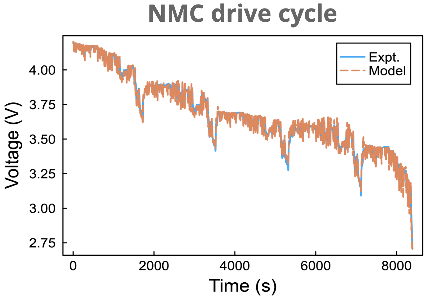
Drive cycle setup
Drive cycles are vital for accurate battery modeling, simulating real-world scenarios and behaviors in vehicle usage. Engineers utilize drive cycles to optimize battery designs, evaluate degradation patterns, and enhance efficiency for electric vehicles and grid storage. Understanding battery behavior relies on the insights provided by drive cycles.
To simulate a drive cycle with JuliaSim Batteries, first build a function that interpolates the drive cycle data. The drive_cycle function should take a time as an input and return the current at that time.
using JuliaSimBatteries
cell = DFN(NMC())

expt = current((u, p, t) -> drive_cycle(t))

sol = solve(cell, expt, SOC_initial = 1)
The plot below shows agreement with experimental agreement with an NMC cell.